Author Archives: John Salatas

Automating the creation of joint multigram language models as WFST: Part 2

(originally posted at http://cmusphinx.sourceforge.net/2012/06/automating-the-creation-of-joint-multigram-language-models-as-wfst-part-2/)

Foreword

This a article presents an updated version of the model training application originally discussed in [1], considering the compatibility issues with phonetisaurus decoder as presented in [2]. The updated code introduces routines to regenerate a new binary fst model compatible with phonetisaurus’ decoder as suggested in [2] which will be reviewed in the next section.

1. Code review

The basic code for the model regeneration is defined in train.cpp in procedure

1
void relabel(StdMutableFst *fst, StdMutableFst *out, string eps, string skip, string s1s2_sep, string seq_sep);

where fst and out are the input and output (the regenerated) models respectively.

In the first initialization step is to generate new input, output and states SymbolTables and add to output the new start and final states [2].

Furthermore, in this step the SymbolTables are initialized. Phonetisauruss decoder requires the symbols   eps, seq_sep, “<phi>”, “<s>” and “<s>” to be in keys 0, 1, 2, 3, 4 accordingly.

1
2
3
4
5
6
7
8
9
10
11
12
13
14
15
16
17
18
19
20
21
22
23
24
25
26
27
28
29
30
31
32
33
34
35
36
37
void relabel(StdMutableFst *fst, StdMutableFst *out, string eps, string skip, string s1s2_sep, string seq_sep) {
	ArcSort(fst, StdILabelCompare());
	const SymbolTable *oldsyms = fst->InputSymbols();
 
	// Uncomment the next line in order to save the original model
	// as created by ngram
	// fst->Write("org.fst");
	// generate new input, output and states SymbolTables
	SymbolTable *ssyms = new SymbolTable("ssyms");
	SymbolTable *isyms = new SymbolTable("isyms");
	SymbolTable *osyms = new SymbolTable("osyms");
 
	out->AddState();
	ssyms->AddSymbol("s0");
	out->SetStart(0);
 
	out->AddState();
	ssyms->AddSymbol("f");
	out->SetFinal(1, TropicalWeight::One());
 
	isyms->AddSymbol(eps);
	osyms->AddSymbol(eps);
 
	//Add separator, phi, start and end symbols
	isyms->AddSymbol(seq_sep);
	osyms->AddSymbol(seq_sep);
	isyms->AddSymbol("<phi>");
	osyms->AddSymbol("<phi>");
	int istart = isyms->AddSymbol("<s>");
	int iend = isyms->AddSymbol("</s>");
	int ostart = osyms->AddSymbol("<s>");
	int oend = osyms->AddSymbol("</s>");
 
	out->AddState();
	ssyms->AddSymbol("s1");
	out->AddArc(0, StdArc(istart, ostart, TropicalWeight::One(), 2));
	...

In the main step, the code iterates through each State of the input model and adds each one to the output model keeping track of old and new state_id in ssyms SymbolTable.

In order to transform to an output model with a single final state [2] the code checks if the current state is final and if it is, it adds an new arc connecting from the current state to the single final one (state_id 1) with label “</s>:</s>” and weight equal to the current state’s final weight. It also sets the final weight of current state equal to TropicalWeight::Zero() (ie it converts the current state to a non final).

1
2
3
4
5
6
7
8
9
10
11
12
13
14
15
16
17
18
19
20
21
22
23
24
25
26
27
28
29
30
31
	...
	for (StateIterator<StdFst> siter(*fst); !siter.Done(); siter.Next()) {
		StateId state_id = siter.Value();
 
		int64 newstate;
		if (state_id == fst->Start()) {
			newstate = 2;
		} else {
			newstate = ssyms->Find(convertInt(state_id));
			if(newstate == -1 ) {
				out->AddState();
				ssyms->AddSymbol(convertInt(state_id));
				newstate = ssyms->Find(convertInt(state_id));
			}
		}
 
		TropicalWeight weight = fst->Final(state_id);
 
		if (weight != TropicalWeight::Zero()) {
			// this is a final state
			StdArc a = StdArc(iend, oend, weight, 1);
			out->AddArc(newstate, a);
			out->SetFinal(newstate, TropicalWeight::Zero());
		}
		addarcs(state_id, newstate, oldsyms, isyms, osyms, ssyms, eps, s1s2_sep, fst, out);
	}
	out->SetInputSymbols(isyms);
	out->SetOutputSymbols(osyms);
	ArcSort(out, StdOLabelCompare());
	ArcSort(out, StdILabelCompare());
}

Lastly, the addarcs procuder is called in order to relabel the arcs of each state of the input model and add them to the output model. It also creates any missing states (ie missing next states of an arc).

1
2
3
4
5
6
7
8
9
10
11
12
13
14
15
16
17
18
19
20
21
22
23
24
25
void addarcs(StateId state_id, StateId newstate, const SymbolTable* oldsyms, SymbolTable* isyms,
		SymbolTable* osyms,	SymbolTable* ssyms,	string eps,	string s1s2_sep, StdMutableFst *fst,
		StdMutableFst *out) {
	for (ArcIterator<StdFst> aiter(*fst, state_id); !aiter.Done(); aiter.Next()) {
		StdArc arc = aiter.Value();
		string oldlabel = oldsyms->Find(arc.ilabel);
		if(oldlabel == eps) {
			oldlabel = oldlabel.append("}");
			oldlabel = oldlabel.append(eps);
		}
		vector<string> tokens;
		split_string(&oldlabel, &tokens, &s1s2_sep, true);
		int64 ilabel = isyms->AddSymbol(tokens.at(0));
		int64 olabel = osyms->AddSymbol(tokens.at(1));
 
		int64 nextstate = ssyms->Find(convertInt(arc.nextstate));
		if(nextstate  == -1 ) {
			out->AddState();
			ssyms->AddSymbol(convertInt(arc.nextstate));
			nextstate = ssyms->Find(convertInt(arc.nextstate));
		}
		out->AddArc(newstate, StdArc(ilabel, olabel, (arc.weight != TropicalWeight::Zero())?arc.weight:TropicalWeight::One(), nextstate));
		//out->AddArc(newstate, StdArc(ilabel, olabel, arc.weight, nextstate));
	}
}

2. Performance – Evaluation

In order to evaluate the perfomance of the model generated with the new code. A new model was trained  with the same dictionaries as in [4]

# train/train --order 9 --smooth "kneser_ney" --seq1_del --seq2_del --ifile cmudict.dict.train  --ofile cmudict.fst

and evaluated with phonetisaurus evaluate script

# evaluate.py --modelfile cmudict.fst --testfile ../cmudict.dict.test --prefix cmudict/cmudict
Mapping to null...
Words: 13335  Hyps: 13335 Refs: 13335
######################################################################
EVALUATION RESULTS
----------------------------------------------------------------------
(T)otal tokens in reference: 84993
(M)atches: 77095  (S)ubstitutions: 7050  (I)nsertions: 634  (D)eletions: 848
% Correct (M/T)           -- %90.71
% Token ER ((S+I+D)/T)    -- %10.04
% Accuracy 1.0-ER         -- %89.96
--------------------------------------------------------
(S)equences: 13335  (C)orrect sequences: 7975  (E)rror sequences: 5360
% Sequence ER (E/S)       -- %40.19
% Sequence Acc (1.0-E/S)  -- %59.81
######################################################################

3. Conclusions – Future work

The evaluation results in cmudict dictionary, are a little bit worst than using the command line procedure in [4]. Although the difference doesn’t seem to be important, it needs a further investigation. For that purpose and for general one can uncomment the line fst->Write(“org.fst”); in the relabel procedure as depicted in a previous section, in order to have the original binary model saved in a file called “org.fst”.

Next steps would probably be to write code in order to load the binary model in java code and to port the decoding algorithm along with the required fst operations to java and eventually integrate it with CMUSphinx.

References
[1] J. Salatas, “Automating the creation of joint multigram language models as WFST”, ICT Research Blog, June 2012.
[2] J. Salatas, Compatibility issues using binary fst models generated by OpenGrm NGram Library with phonetisaurus decoder”, ICT Research Blog, June 2012.
[3] fstinfo on models created with opengrm
[4] J. Salatas, Using OpenGrm NGram Library for the encoding of joint multigram language models as WFST”, ICT Research Blog, June 2012.

Compatibility issues using binary fst models generated by OpenGrm NGram Library with phonetisaurus decoder

(originally posted at http://cmusphinx.sourceforge.net/2012/06/compatibility-issues-using-binary-fst-models-generated-by-opengrm-ngram-library-with-phonetisaurus-decoder/)

Foreword

Previous articles have shown how to use OpenGrm NGram Library for the encoding of joint multigram language models as WFST [1] and provided the code that simplifies and automates the fst model training [2]. As described in [1] the generated binary fst models with the procedures described in those articles are not directly usable from phonetisaurus [3] decoder.

This article will try to describe the compatibility issues in more details and provide some intuition on possible solutions and workarounds.

1. Open issues

Assuming a binary fst model, named cmudict.fst generated as described in [1], trying to evaluate it with phonetisaurus evaluate python script, results in the following error

$ ./evaluate.py --order 9 --modelfile cmudict.fst --testfile cmudict.dict.test.tabbed --prefix cmudict/cmudict
../phonetisaurus-g2p --model=cmudict.fst --input=cmudict/cmudict.words --beam=1500 --alpha=0.6500 --prec=0.8500 --ratio=0.7200 --order=9 --words --isfile  > cmudict/cmudict.hyp
Symbol: 'A' not found in input symbols table.
Mapping to null...
Symbol: '4' not found in input symbols table.
Mapping to null...
Symbol: '2' not found in input symbols table.
Mapping to null...
Symbol: '1' not found in input symbols table.
Mapping to null...
Symbol: '2' not found in input symbols table.
Mapping to null...
Symbol: '8' not found in input symbols table.
Mapping to null...
sh: line 1: 18788 Segmentation fault      ../phonetisaurus-g2p --model=cmudict.fst --input=cmudict/cmudict.words --beam=1500 --alpha=0.6500 --prec=0.8500 --ratio=0.7200 --order=9 --words --isfile > cmudict/cmudict.hyp
Words: 0  Hyps: 0 Refs: 13328
Traceback (most recent call last):
File "./evaluate.py", line 124, in <module>
mbrdecode=args.mbrdecode, beam=args.beam, alpha=args.alpha, precision=args.precision, ratio=args.ratio, order=args.order
File "./evaluate.py", line 83, in evaluate_testset
PERcalculator.compute_PER_phonetisaurus( hypothesisfile, referencefile, verbose=verbose )
File "calculateER.py", line 333, in compute_PER_phonetisaurus
assert len(words)==len(hyps) and len(hyps)==len(refs)
AssertionError

2. Disussion on open issues

In order to investigate the error above, a simple aligned corpus was created as below

a}a b}b
a}a
a}a c}c
a}a b}b c}c
a}a c}c
b}b c}c

This simple corpus was used as input to both ngram and phonetisaurus model training procedures [1], [3] and the generated fst model (binary.fst) was visualized as follows

$ fstdraw binary.fst binary.dot
$ dot -Tps binary.dot > binary.ps

the generated two postscript outputs, using phonetisaurus and ngram respectively, are shown in the following figures:

Visualization of the fst model generated by phonetisaurus

Figure 1: Visualization of the fst model generated by phonetisaurus

Visualization of the fst model generated by ngram

Figure 2: Visualization of the fst model generated by ngram

By studying the two figures above the first obvious conclusion is that the model generated with ngram do not distinguish between graphemes (input label) and phonemes (output label), but it uses the joint multigram (eg “a}a”) as both input and output label.

Another obvious difference between the two models is the starting and final state(s). Phonetisaurus models have a fixed starting state with a single outgoing arc with labels <s>:<s> and no weight. Furthermore, in phonetisaurus model there exist only a single final state with </s>:</s> labels in all incoming arcs.

3. Possible solutions and workarounds

[1] already presents a workaround to bypass the compatibility issues described in the previous section. We can simply export the ngram generated binary fst model to an ARPA format with:

$ ngramprint --ARPA binary.fst > export.arpa

and the use phonetisaurus’ arpa2fst convert utility to regenerate a new binary fst model compatible with phonetisaurus’ decoder.

$ phonetisaurus-arpa2fst –input=export.arpa

Although this is a straightforward procedure, a  more elegant solution would be to iterate in all arcs and manually break apart the grapheme/phoneme joint multigram labels to input/output labels accordingly. A final step, if necessary, would be to add the start and single final state in the ngram generated fst model.

4. Conclusion – Future work

This article tried to provide some intuition on the compatibility issues between ngram and phonetisaurus models and also to possible solutions and workarounds. As explained in the previous section, there is already a straightforward procedure to overcome these issues (export to ARPA format and regenerate the binary model), but in any case it is worth to try the relabeling approach described also in the previous section.

References

[1] J. Salatas, “Using OpenGrm NGram Library for the encoding of joint multigram language models as WFST”, ICT Research Blog, June 2012.

[2] J. Salatas, “Automating the creation of joint multigram language models as WFST”, ICT Research Blog, June 2012.

[3] J. Salatas, “Phonetisaurus: A WFST-driven Phoneticizer – Framework Review”, ICT Research Blog, June 2012.

Automating the creation of joint multigram language models as WFST

Notice: This article is outdated. The application described here is now part of the SphinxTrain application. Please refer to recent articles in CMUSphinx category for the latest info.

(originally posted at http://cmusphinx.sourceforge.net/2012/06/automating-the-creation-of-joint-multigram-language-models-as-wfst/)

Foreword

Previous articles have introduced the C++ code to align a pronounciation dictionary [1] and how this aligned dictionary can be used in combination with OpenGrm Ngram Library for the encoding of joint multigram language models as WFST [2]. This article will describe the automation of the language model creation procedures as a complete C++ application that is simpler to use than the original procedures described in [2].

1. Installation
The procedure below is tested on an Intel CPU running openSuSE 12.1 x64 with gcc 4.6.2. Further testing is required for other systems (MacOSX, Windows).

The code requires the openFST library to be installed on your system. Having downloaded, compiled and installed openFST, the first step is to checkout the code from the cmusphinx SVN repository:

$ svn co https://cmusphinx.svn.sourceforge.net/svnroot/cmusphinx/branches/g2p/train

and compile it

$ cd train
$ make
g++ -c -g -o src/train.o src/train.cpp
g++ -c -g -o src/phonetisaurus/M2MFstAligner.o src/phonetisaurus/M2MFstAligner.cpp
g++ -c -g -o src/phonetisaurus/FstPathFinder.o src/phonetisaurus/FstPathFinder.cpp
g++ -g -L/usr/local/lib64/fst -lfst -lfstfar -lfstfarscript -ldl -lngram -o train src/train.o src/phonetisaurus/M2MFstAligner.o src/phonetisaurus/FstPathFinder.o
$

2. Usage
Having compiled the script, running it without any command line arguments will print out it’s usage:
$ ./train
Input file not provided
Usage: ./train [--seq1_del] [--seq2_del] [--seq1_max SEQ1_MAX] [--seq2_max SEQ2_MAX]
[--seq1_sep SEQ1_SEP] [--seq2_sep SEQ2_SEP] [--s1s2_sep S1S2_SEP]
[--eps EPS] [--skip SKIP] [--seq1in_sep SEQ1IN_SEP] [--seq2in_sep SEQ2IN_SEP]
[--s1s2_delim S1S2_DELIM] [--iter ITER] [--order ORDER] [--smooth SMOOTH]
[--noalign] --ifile IFILE --ofile OFILE
--seq1_del, Allow deletions in sequence 1. Defaults to false.
--seq2_del, Allow deletions in sequence 2. Defaults to false.
--seq1_max SEQ1_MAX, Maximum subsequence length for sequence 1. Defaults to 2.
--seq2_max SEQ2_MAX, Maximum subsequence length for sequence 2. Defaults to 2.
--seq1_sep SEQ1_SEP, Separator token for sequence 1. Defaults to '|'.
--seq2_sep SEQ2_SEP, Separator token for sequence 2. Defaults to '|'.
--s1s2_sep S1S2_SEP, Separator token for seq1 and seq2 alignments. Defaults to '}'.
--eps EPS, Epsilon symbol. Defaults to ''.
--skip SKIP, Skip/null symbol. Defaults to '_'.
--seq1in_sep SEQ1IN_SEP, Separator for seq1 in the input training file. Defaults to ''.
--seq2in_sep SEQ2IN_SEP, Separator for seq2 in the input training file. Defaults to ' '.
--s1s2_delim S1S2_DELIM, Separator for seq1/seq2 in the input training file. Defaults to ' '.
--iter ITER, Maximum number of iterations for EM. Defaults to 10.
--ifile IFILE, File containing training sequences.
--ofile OFILE, Write the binary fst model to file.
--noalign, Do not align. Assume that the aligned corpus already exists.
Defaults to false.
--order ORDER, N-gram order. Defaults to 9.
--smooth SMOOTH, Smoothing method. Available options are:
"presmoothed", "unsmoothed", "kneser_ney", "absolute",
"katz", "witten_bell", "unsmoothed". Defaults to "kneser_ney".
$

As in [1], the two required options are the pronunciation dictionary (IFILE) and the file in which the binary fst model will be saved (OFILE). The script provide default values for all other options and an fst binary model for cmudict (v. 0.7a) can be created simply by the following command

$ ./train --seq1_del --seq2_del --ifile <path to cmudict> --ofile <path to binary fst>

allowing for deletions in both graphemes and phonemes, and

$ ./train --ifile <path to cmudict> --ofile <path to binary fst>

not allowing for deletions.

3. Performance, Evaluation and Comparison with phonetisaurus
in order to test the new code’s performance, tests similar to those in [1] and [2] where performed, with similar results in both resource utilization and it’s ability to generate pronunciations for previously unseen words.

4. Conclusion – Future Works
Having integrated the model training procedure into a simplified application, combined with the dictionary alignment code, the next step would be to create the evaluation code in order to avoid using phonetisaurus evaluate python script. Further steps include the writing of the necessary code to load the WFST binary model in java code, and convert it to the java’s implementation of openFST [3], [4].

References
[1] J. Salatas, “Porting phonetisaurus many-to-many alignment python script to C++”, ICT Research Blog, May 2012.
[2] J. Salatas, “Using OpenGrm NGram Library for the encoding of joint multigram language models as WFST”, ICT Research Blog, June 2012.
[3] J. Salatas, “Porting openFST to java: Part 1”, ICT Research Blog, May 2012.
[4] J. Salatas, “Porting openFST to java: Part 2”, ICT Research Blog, May 2012.

Using OpenGrm NGram Library for the encoding of joint multigram language models as WFST

(originally posted at http://cmusphinx.sourceforge.net/2012/06/using-opengrm-ngram-library-for-the-encoding-of-joint-multigram-language-models-as-wfst/)

Foreword
This article will review the OpenGrm NGram Library [1] and its usage for language modeling in ASR. OpenGrm makes use of functionality in the openFST library [2] to create, access and manipulate n-gram language models and it can be used as the language model training toolkit for integrating phonetisaurus’ model training procedures [3] into a simplified application.

1. Model Training
Having the aligned corpus produced from cmudict by the aligner code of our previous article [4], the first step is to generate an OpenFst-style symbol table for the text tokens in input corpus. This can be done with: [5]

# ngramsymbols < cmudict.corpus > cmudict.syms

Given the symbol table, a text corpus can be converted to a binary finite state archive (far) [6] with:

# farcompilestrings --symbols=cmudict.syms --keep_symbols=1 cmudict.corpus > cmudict.far

Next step is to count n-grams from an input corpus, converted in FAR format. It produces an n-gram model in the FST format. By using the switch –order the maximum length n-gram to count can be chosen.

The 1-gram through 9-gram counts for the cmudict.far finite-state archive file created above can be created with:

# ngramcount --order=9 cmudict.far > cmudict.cnts

Finally the 9-gram counts in cmudict.cnts above can be converted to a WFST model with:

# ngrammake --method="kneser_ney" cmudict.cnts > cmudict.mod

The –method option is used for selecting the smoothing method [7] from one of the six available:

  • witten_bell: smooths using Witten-Bell [8], with a hyperparameter k, as presented in [9].
  • absolute: smooths based on Absolute Discounting [10], using bins and discount parameters.
  • katz: smooths based on Katz Backoff [11], using bins parameters.
  • kneser_ney: smooths based on Kneser-Ney [12], a variant of Absolute Discounting.
  • presmoothed: normalizes at each state based on the n-gram count of the history.
  • unsmoothed: normalizes the model but provides no smoothing.

2. Evaluation – Comparison with phonetisaurus

In order to evaluate OpenGrm models, ther procedure described above was repeated using the standard 90%-10% split of the cmudict into a training and test set respectively. The binary fst format produced by ngrammake wasn’t readable by the phonetisaurus evaluation script, so it was converted to ARPA format with:

# ngramprint --ARPA cmudict.mod > cmudict.arpa

and then back to a phonetisaurus binary fst format with:

# phonetisaurus-arpa2fst --input=cmudict.arpa --prefix="cmudict/cmudict"

Finally the test set was evaluated with

# evaluate.py --modelfile cmudict/cmudict.fst --testfile cmudict.dict.test --prefix cmudict/cmudict
Words: 13328 Hyps: 13328 Refs: 13328
##############################################
EVALUATION RESULTS
---------------------------------------------------------------------
(T)otal tokens in reference: 84955
(M)atches: 77165 (S)ubstitutions: 7044 (I)nsertions: 654 (D)eletions: 746
% Correct (M/T) -- %90.83
% Token ER ((S+I+D)/T) -- %9.94
% Accuracy 1.0-ER -- %90.06
---------------------------------------------------------------------
(S)equences: 13328 (C)orrect sequences: 8010 (E)rror sequences: 5318
% Sequence ER (E/S) -- %39.90
% Sequence Acc (1.0-E/S) -- %60.10
##############################################

3. Conclusion – Future Works

The evaluation results above are, as expected, almost identical with those produced by the phonetisaurus’ procedures and the use of MITLM toolkit instead of OpenGrm.

Having the above description, the next step is to integrate all of the commands above into a simplified application, combined with the dictionary alignment code introduced in our previous article [13].

References

[1] OpenGrm NGram Library

[2] openFST library

[3] “Phonetisaurus: A WFST-driven Phoneticizer – Framework Review”, ICT Research Blog, May 2012.

[4] “Porting phonetisaurus many-to-many alignment python script to C++”, ICT Research Blog, May 2012.

[5] OpenGrm NGram Library Quick Tour

[6] OpenFst Extensions: FST Archives (FARs)

[7] S.F. Chen, G. Goodman, “An Empirical Study of Smoothing Techniques for Language Modeling”, Harvard Computer Science Technical report TR-10-98, 1998.

[8] I. H. Witten, T. C. Bell, “The zero-frequency problem: Estimating the probabilities of novel events in adaptive text compression”, IEEE Transactions on Information Theory 37 (4), pp. 1085–1094, 1991.

[9] B. Carpenter, “Scaling high-order character language models to gigabytes”, Proceedings of the ACL Workshop on Software, pp. 86–99, 2005.

[10] H. Ney, U. Essen, R. Kneser, “On structuring probabilistic dependences in stochastic language modeling”, Computer Speech and Language 8, pp. 1–38, 1994.

[11] S. M. Katz, “Estimation of probabilities from sparse data for the language model component of a speech recogniser”, IEEE Transactions on Acoustics, Speech, and Signal Processing 35 (3), pp. 400–401, 1987.

[12] R. Kneser, H. Ney, “Improved backing-off for m-gram language modeling”, Proceedings of the IEEE International Conference on Acoustics, Speech, and Signal Processing (ICASSP). pp. 181–184, 1995.

[13] Porting phonetisaurus many-to-many alignment python script to C++

Porting phonetisaurus many-to-many alignment python script to C++

Notice: This article is outdated. The application described here is now part of the SphinxTrain application. Please refer to recent articles in CMUSphinx category for the latest info.

(originally posted at http://cmusphinx.sourceforge.net/2012/05/porting-phonetisaurus-many-to-many-alignment-python-script-to-c/)

Foreword

Following our previous article on phonetisaurus [1] and the decision to use this framework as the g2p conversion method for my GSoC project, this article will describe the port of the dictionary alignment script to C++.

1. Installation
The procedure below is tested on an Intel CPU running openSuSE 12.1 x64 with gcc 4.6.2. Further testing is required for other systems (MacOSX, Windows).

The alignment script requires the openFST library [2] to be installed on your system. Having downloaded, compiled and installed openFST, the first step is to checkout the alignment code from the cmusphinx SVN repository:

$ svn co https://cmusphinx.svn.sourceforge.net/svnroot/cmusphinx/branches/g2p/train

and compile it

$ cd train
$ make
g++ -c -g -o src/align.o src/align.cpp
g++ -c -g -o src/phonetisaurus/M2MFstAligner.o src/phonetisaurus/M2MFstAligner.cpp
g++ -c -g -o src/phonetisaurus/FstPathFinder.o src/phonetisaurus/FstPathFinder.cpp
g++ -g -l fst -l dl -o src/align src/align.o src/phonetisaurus/M2MFstAligner.o src/phonetisaurus/FstPathFinder.o
$

2. Usage
Having compiled the script, running it without any command line arguments will print out it’s usage, which is similar to that of the original phonetisaurus m2m-aligner python script:
$ cd src
$ ./align
Usage: ./align [--seq1_del] [--seq2_del] [--seq1_max SEQ1_MAX] [--seq2_max SEQ2_MAX]
[--seq1_sep SEQ1_SEP] [--seq2_sep SEQ2_SEP] [--s1s2_sep S1S2_SEP]
[--eps EPS] [--skip SKIP] [--seq1in_sep SEQ1IN_SEP] [--seq2in_sep SEQ2IN_SEP]
[--s1s2_delim S1S2_DELIM] [--iter ITER] --ifile IFILE --ofile OFILE
--seq1_del, Allow deletions in sequence 1. Defaults to false.
--seq2_del, Allow deletions in sequence 2. Defaults to false.
--seq1_max SEQ1_MAX, Maximum subsequence length for sequence 1. Defaults to 2.
--seq2_max SEQ2_MAX, Maximum subsequence length for sequence 2. Defaults to 2.
--seq1_sep SEQ1_SEP, Separator token for sequence 1. Defaults to '|'.
--seq2_sep SEQ2_SEP, Separator token for sequence 2. Defaults to '|'.
--s1s2_sep S1S2_SEP, Separator token for seq1 and seq2 alignments. Defaults to '}'.
--eps EPS, Epsilon symbol. Defaults to ''.
--skip SKIP, Skip/null symbol. Defaults to '_'.
--seq1in_sep SEQ1IN_SEP, Separator for seq1 in the input training file. Defaults to ''.
--seq2in_sep SEQ2IN_SEP, Separator for seq2 in the input training file. Defaults to ' '.
--s1s2_delim S1S2_DELIM, Separator for seq1/seq2 in the input training file. Defaults to ' '.
--iter ITER, Maximum number of iterations for EM. Defaults to 10.
--ifile IFILE, File containing sequences to be aligned.
--ofile OFILE, Write the alignments to file.
$

The two required options are the pronunciation dictionary to align (IFILE) and the file in which the aligned corpus will be saved (OFILE). The script provide default values for all other options and cmudict (v. 0.7a) can be aligned simply by the following command
$ ./align --seq1_del --seq2_del --ifile <path to cmudict> --ofile <path to aligned corpus>

allowing for deletions in both graphemes and phonemes, and

$ ./align --ifile <path to cmudict> --ofile <path to aligned corpus>

not allowing for deletions.

3. Performance

In order to test the new alignment script’s performance in both its results and its requirements for cpu and memory usage, I have performed two tests for aligning of the full cmudict (v. 0.7a) allowing deletions in both sequenses:

$ ./align --seq1_del --seq2_del --ifile ../data/cmudict.dict --ofile ../data/cmudict.corpus.gsoc

and compared with the original phonetisuarus script

$ ./m2m-aligner.py --align ../train/data/cmudict.dict -s2 -s1 --write_align ../train/data/cmudict.corpus

3.1. Alignment

Comparing of the two outputs using the linux diff util, didn’t result in major differences. Minor differences were noticed in case of the alignment double vowels and consonants with a single phoneme, as in the two following examples:

--- cmudict.corpus
+++ cmudict.corpus.gsoc
....
-B}B O}AO1 R}_ R}R I}IH0 S}S
+B}B O}AO1 R}R R}_ I}IH0 S}S
....
-B}B O}AO1 S|C}SH H}_ E}_ E}IY0
+B}B O}AO1 S|C}SH H}_ E}IY0 E}_
....

3.2. CPU memory usage

In the system described above, the average (of two runs) running time for new aligned command was 1h:14m in comparison to an average of 1h:28m of the original phonetisaurus script. Both scripts consumed the same RAM amount (~ 1.7GB).

Conclusion – Future works

This article presented the new g2p align script which seems to produce the same results as the original one and is a little bit faster than that.

Although it should compile and run as expected to any modern linux system, further testing is reeuired for other systems (like MacOSX, windows). We need also to investigated the alignment differnces (compared to the original script) in the vowels and consonants as described above. Although it doesn’t seem critical, it may cause problems later.

References

[1] J. Salatas, “Phonetisaurus: A WFST-driven Phoneticizer – Framework Review”, ICT Research Blog, May 2012.

[2] OpenFst Library

Porting openFST to java: Part 2

Notice: Parts of this article may be outdated. There are many changes to its API and performance improvements recently in the java fst framework. Please refer to recent articles in Java FST Framework category for the latest info.

(originally posted at http://cmusphinx.sourceforge.net/2012/05/porting-openfst-to-java-part-2/)

Foreword

This article, the second in a series regarding, porting openFST to java, briefly presents some additional base classes and raise some issues regarding the java fst architecture in general and its compatibility with the original openFST binary format for saving models.

1. FST java library base architecture
The first article in the series [1] introduced the Weight<T> class, the semiring operations related classes and interfaces and finally a solid class implementation for the tropical semiring based on float weights. In the last svn commit (revision 11363) [2] includes the edu.cmu.sphinx.fst.weight.LogSemiring class which implements a logarithmic semiring based on Double weight values.

Furthermore revision 11363 includes the edu.cmu.sphinx.fst.state.State<W extends Weight<?>>, edu.cmu.sphinx.fst.arc.Arc<W extends Weight<?>> and edu.cmu.sphinx.fst.fst.Fst<W extends Weight<?>> classes which implement the state, arc and fst functionality, respectively.

2. Architecture design issues

2.1. Java generics support

As described in the first part [1], the edu.cmu.sphinx.fst.weight.Weight<T> acts basically as a wrapper for the weight’s value. The current implementation of State, Arc and Fst classes take as a type parameter any class that extends the Weight base class. Although this approach provides a great flexibility on building custom types of FSTs, the implementations can be greatly simplified if we assume only the base Weight class and modify the State, Arc and Fst classes definition to simply use a type parameter.

As an example the Arc class definition would be simplified to

1
2
3
4
5
6
7
8
public class Arc<T> implements Serializable{
 
	private static final long serialVersionUID = -7996802366816336109L;
 
	// Arc's weight
	protected Weight<T> weight;
	// Rest of the code.....
}

instead of its current definition

1
2
3
4
5
6
7
8
public class Arc<W extends Weight<?>> implements Serializable{
 
	private static final long serialVersionUID = -7996802366816336109L;
 
	// Arc's weight
	protected W weight;
	// Rest of the code.....
}

The proposed modification can be applied also to State and Fst classes and provide an easier to use api. In that case the construction of a basic FST in the class edu.cmu.sphinx.fst.demos.basic.FstTest would be simplified as follows

1
2
3
4
5
6
7
8
9
10
11
12
13
14
15
16
17
18
// ...
Fst<Double> fst = new Fst<Double>();
 
// State 0
State<Double> s = new State<Double>(); 
s.AddArc(new Arc<Double>(new Weight<Double>(0.5), 1, 1, 1));
s.AddArc(new Arc<Double>(new Weight<Double>(1.5), 2, 2, 1));
fst.AddState(s);
 
// State 1
s = new State<Double>();
s.AddArc(new Arc<Double>(new Weight<Double>(2.5), 3, 3, 2));
fst.AddState(s);
 
// State 2 (final)
s = new State<Double>(new Weight<Double>(3.5));
fst.AddState(s);
// ...

The code could be further simplified by completely dropping generics support in State, Arc and Fst classes by just providing solid implementations based on Weight weights.

2.2. Compatibility with the original openFST binary format

A second issue is the compatibility of the serialized binary format with the original openFST format. A compatible java library that is able to load/save openFST models, would provide us the ability to share trained models between various applications. As an example, in the case of ASR applications, trained models could be easily shared between between sphinx4 and kaldi [3] which is written in C++ and already uses the openFST library.

References

[1] J. Salatas, “Porting openFST to java: Part 1”, ICT Research Blog, May 2012.

[2] CMUSphinx g2p SVN repository

[3] Kaldi Speech recognition research toolkit , last accessed: 18/05/2012.

[4] C. Allauzen, M. Riley, J. Schalkwyk, W. Skut, M. Mohri, “OpenFst: a general and efficient weighted finite-state transducer library”, Proceedings of the 12th International Conference on Implementation and Application of Automata (CIAA 2007), pp. 11–23, Prague, Czech Republic, July 2007.

Porting openFST to java: Part 1

Notice: Parts of this article may be outdated. There are many changes to its API and performance improvements recently in the java fst framework. Please refer to recent articles in Java FST Framework category for the latest info.

Foreword

This article is the first part of a series of articles on porting openFST[1] in java. OpenFST is an open-source C++ library for weighted finite-state transducers (WFSTs) [1] and having a similar java implementation is a crucial first step for the integration of phonetisaurus g2p into sphinx 4 [2]

This article will briefly review some mathematical background of weighted finite-state transducers  describe the current implementation of openFST and then start describing the java implementation which will be completed in articles that will follow.

1.  Weighted finite-state transducers

Weighted finite-state transducers have been used in speech recognition and synthesis, machine translation, optical character recognition, pattern matching,string processing, machine learning, information extraction and retrieval among others. Having a comprehensive software library of weighted transducer representations and core algorithms is key for using weighted transducers in these applications and for the development of new algorithms and applications. [1]

A weighted finite-state transducer (WFST) is a finite automaton for which each transition has an input label, an output label, and a weight. Figure 1 depicts a weighted finite state transducer: [1]

Figure 1:  Example weighted finite-state transducer

Figure 1: Example weighted finite-state transducer

The initial state is labeled 0. The final state is 2 with final weight of 3.5. Any state with non-infinite final weight is a final state. There is a transition from state 0 to 1 with input label a, output label x, and weight 0.5. This machine transduces, for instance, the string ac to xz with weight 6.5 (the sum of the arc and final weights). [1]

The weights may represent any set so long as they form a semiring. A semiring (\mathbb{K}, \oplus, \otimes, \bar{0}, \bar{1})   is specified by a set of values \mathbb{K} , two binary operations \oplus   and \otimes , and two designated values \bar{0} and \bar{1} . The operation \oplus is associative, commutative, and has  \bar{0} as identity. The operation \otimes is associative, has identity $ and \bar{1} , distributes with respect to \oplus , and has \bar{0} as annihilator: for all a \in \mathbb{K} , a \otimes \bar{0} = \bar{0} \otimes a = \bar{0} . If \otimes is also commutative, we say that the semiring is commutative. [1]

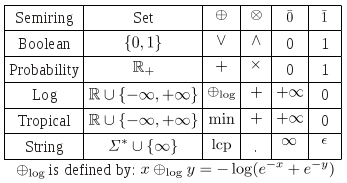
Table 1 below lists some common semirings. All but the last are defined over subsets of the real numbers (extended with positive and negative infinity). In addition to the familiar Boolean semiring, and the probability semiring used to combine probabilities, two semirings often used in applications are the log semiring which is isomorphic to the probability semiring via the negative-log mapping, and the tropical semiring which is similar to the log semiring except the  operation is min. The left (right) string semiring, which is defined over strings, has longest common prefix (suffix) and concatenation as its operations, and has the (extended element) infinite string and the empty string for its identity elements. It only distributes on the left (right). [1]

Table 1:  Semiring examples.

Table 1: Semiring examples.

2.  The openFST C++ library:  Representation and Construction

The motivation for OpenFst was to create a library as comprehensive and efficient as the AT&T FSM [3] Library, but that was an open-source project. We also sought to make this library as flexible and customizable as possible given the wide range of applications WFSTs have enjoyed in recent years. It is a C++ template library, allowing it to be both very customizable and efficient. [1]

In the OpenFst Library, a transducer can be constructed from either the C++ level using class constructors and mutators or from a shell-level program using a textual file representation. [1]

In order to create a transducer using openFST we need first to construct an empty VectorFst: [1]

1
2
// A vector FST is a general mutable FST
VectorFst<StdArc> fst;

The VectorFst, like all transducer representations and algorithms in this library, is templated on the transition type. This permits customization of the labels, state IDs and weights in a transducer. StdArc defines the library-standard transition representation:

1
2
3
4
5
6
7
8
9
10
11
12
13
14
15
16
17
18
19
20
21
22
23
template <class W>
class ArcTpl {
 public:
  typedef W Weight;
  typedef int Label;
  typedef int StateId;
 
  ArcTpl(Label i, Label o, const Weight& w, StateId s)
      : ilabel(i), olabel(o), weight(w), nextstate(s) {}
 
  ArcTpl() {}
 
  static const string &Type(void) {
    static const string type =
        (Weight::Type() == "tropical") ? "standard" : Weight::Type();
    return type;
  }
 
  Label ilabel;
  Label olabel;
  Weight weight;
  StateId nextstate;
};

A Weight class holds the set element and provides the semiring operations. Currently openFST provides many different C++ Template-based implementations like TropicalWeightTpl, LogWeightTpl and MinMaxWeightTpl which extend a base FloatWeightTpl (see float-weight.h for implementation details) and others. Having these Template-based implementations opeFST we need just have a typedef to define a particular Weight such as TropicalWeight:

1
2
// Single precision tropical weight
typedef TropicalWeightTpl<float> TropicalWeight;

3. The proposed FST java library

Based on the above description and on technical implementation differences between C++ and Java, and more specific mostly on a) difference between C++ Templates and Java generics [4] and b) the lack of operation overloads in Java, the initial implementation includes the edu.cmu.sphinx.fst.weight.Weight<T> class, acting basically as a wrapper for the weight’s value, which can be on any type. The Weight<T> class can be extended in order to create more advanced implementations, if needed.

There is also a generics based interface edu.cmu.sphinx.fst.weight.Semiring<W extends Weight<?>> which declares the Plus, Times and Divide semiring operations for a Weight<?> class. In addition, it declares the zero and one elements of the semiring and the boolean isMember(Weight<?> w) method which should be implemented in a way that returns true if w is a member of the semiring  set of values (\mathbb{K} ) or false if it is not. The edu.cmu.sphinx.fst.weight.TropicalSemiring class implements this interface in order to create a solid class of a Tropical Semiring based on single-precision Float type for storing the weight’s values.

Finaly the edu.cmu.sphinx.fst.demos.basic package contains a main class for testing the above functionality by instatiating a TropicalSemiring and performing some operations on various Weight values.

4. Conclusion – Future work

This article tried to describe some basic theoritical background on weighted finite-state transducers, provide a brief description on the openFST architect and foundation classes and finally presented an initial design for the FST java library implementation. Following the general open-source philosophy “perform small commits often” the library is available in CMUShinx’ repository created for the integration of phonetisaurus g2p into sphinx 4. [5]

The next steps is to provide the Arc and Fst classes which over time will be extended to provide the required functionality for the various FST operations needed for my GSoC 2012 project. Hopefully, over time, more functionality will be provided by the community.

References

[1] C. Allauzen, M. Riley, J. Schalkwyk, W. Skut, M. Mohri, “OpenFst: a general and efficient weighted finite-state transducer library”, Proceedings of the 12th International Conference on Implementation and Application of Automata (CIAA 2007), pp. 11–23, Prague, Czech Republic, July 2007.

[2] J. Salatas, “Phonetisaurus: A WFST-driven Phoneticizer – Framework Review”, ICT Research Blog, May 2012.

[3] M. Mohri, F. Pereira, M. Riley, “The Design Principles of a Weighted Finite-State Transducer Library”, Theoretical Computer Science, pp. 15-32, 2000.

[4] H. M. Qusay, “Using and Programming Generics in J2SE 5.0”, Oracle Technology Network, 2004,  last accessed: 08/05/2012.

[5] CMUSphinx g2p SVN repository

Phonetisaurus: A WFST-driven Phoneticizer – Framework Review

Foreword

This article tries to analyze the phonetisaurus g2p [1], [2] code by describing it’s main parts and algorithms behind these. Phonetisaurus is a modular system and includes support for several third-party components. The system has been implemented primarily in python, but also leverages the OpenFST framework [3].

1. Overall Architecture

The procedure for model training and evaluation in phonetisaurus consists by three parts [4]: the dictionary alignment, the model training and finally the evaluation of the model.

1.1. Dictionary Alignment
Manual G2P alignments are generally not available, thus it is necessary to first align the grapheme and phoneme sequences in a pronunciation dictionary, prior to building a pronunciation model. Phonetisaurus utilizes the EM-based many-to-many alignment procedure detailed in [5] that supports alignments from digraphs such as “sh” to a single phoneme, or the reverse case. Recently the dictionary alignment was reimplemented and upgraded using OpenFst.
The command line script that controls the alignment procedure m2m-aligner.py interfaces with the M2MFstAligner class (M2MFstAligner.cpp) using Swig [6], in order to transform two sequences, one of graphemes and one of phonemes to an FST that encodes all possible alignments between the symbols in the two sequences.
The basic transformation of the sequence

1
void M2MFstAligner::Sequences2FST( VectorFst<LogArc>* fst, vector<string>* seq1, vector<string>* seq2 );

creates a VectorFst<LogArc> fst instance and iterates over all possible combinations which are added to the fst. It uitilizes the Plus semiring operation and the Connect optimization operation.

After the FSTs for all entries are created the procedure continus with the EM algorithm which is implemented in the

1
void M2MFstAligner::expectation( );

and

1
float M2MFstAligner::maximization( bool lastiter );

procedures. These procedures utilize the ShortestDistance search operation and the Divide, Times and Plus semiring operations.

1.2. Model Training

The command line script that controls the model training procedure train-model.py uses the estimate-ngram utility of the MIT Language Modeling (MITLM) toolkit [7] in order to estimate an n-gram language model language model by cumulating n-gram count statistics,”smoothing observed counts, and building a backoff n-gram mode [8].
The estimate-ngramm utility produces a language model in ARPA format which is then converted to a FST textual represantion through the use of the arpa2fst.py script. This textual represantion is then parsed by the fstcompile command line utility of OpenFST and converted to the final binary representation.

1.3. Model Evaluation

The command line script that controls the model evaluation procedure evaluate.py utilizes the Phonetisaurus class (Phonetisaurus.cpp), through the phonetisaurus-g2p command line interface, for the g2p conversion, which is then evaluated. It uitilizes the Compose binary operation, Project unary operation, ShortestPath search operation, Times semiring operation and RmEpsilon optimization operation.
A pronunciation for a new word is achieved by compiling the word into a WFSA and composing it with the pronunciation model. The best hypothesis is just the shortest path through the composed WFST. [1]
The input word is converted to an acceptor I which has one arc for each of the characters in the word. I is then composed with M according to O = I ◦ M where ◦ denotes the composition operator. The n-best paths are extracted from O by projecting the output, removing the epsilon labels and applying the n-shortest paths algorithm with determinization. [2]

2. Conclusion – Future Work

This article tried to analyze the phonetisaurus g2p code and its main parts. Having this description will allow us to produce a more accurate and analytical planning and scheduling the tasks required for the integration of phonetisaurus g2p into sphinx 4 for my GSoC 2012 project [9].

References

[1] J. Novak, D. Yang, N. Minematsu, K. Hirose, “Initial and Evaluations of an Open Source WFST-based Phoneticizer”, The University of Tokyo, Tokyo Institute of Technology

[2] D. Yang, et. al., “Rapid development of a G2Psystem based on WFST framework”, ASJ 2009
Autumn session, pp. 111-112, 2009.

[3] C. Allauzen, M. Riley, J. Schalkwyk, W. Skut, M. Mohri, “OpenFst: a general and efficient weighted finite-state transducer library”, Proceedings of the 12th International Conference on Implementation and Application of Automata (CIAA 2007), pp. 11–23, Prague, Czech Republic, July 2007.

[4] J. Novak, README.txt, phonetisaurus source code, last accessed: 29/04/2012.

[5] S. Jiampojamarn, G. Kondrak, T. Sherif, “Applying Many-to-Many Alignments and Hidden Markov Models to Letter-to-Phoneme Conversion”, NAACL HLT, pp. 372-379, 2007.

[6] Simplified Wrapper and Interface Generator, last accessed: 29/04/2012.

[7] MIT Language Modeling Toolkit, last accessed: 29/04/2012.

[8] D. Jurafsky, J. H. Martin, “Speech and Language Processing”, Prentice Hall, 2000.

[9] J. Salatas, GSoC 2012 Project: Letter to Phoneme Conversion in sphinx4, April 2012.

Letter to Phoneme Conversion in CMU Sphinx-4: Literature review

1. Foreword
Currently Sphinx-4 uses a predefined dictionary for mapping words to sequence of phonemes. I propose modifications in the Sphinx-4 code that will enable it to use trained models (through some king of machine learning algorithm) to map letters to phonemes and thus map words to sequence of phonemes without the need of a predefined dictionary. A dictionary will be only used to train the required models.

2. Literature Review
2.1. Grapheme-to-Phoneme methods
Grapheme to Phoneme (G2P) (or Letter to Sound – L2S) conversion is an active research field with applications to both text-to-speech (TTS) and automated speech recognition (ASR) systems. There are many different approaches used for the G2P conversion proposed by different researchers.
Hein [1] proposes a method that use a feedforward neural network for the G2P conversion process and proposes a simple algorithm for the creation of the grapheme-to-phoneme matching database with a phonetic dictionary as input. The method has been tested in both English and German languages. 99.2% of 305000 entries of the German CELEX could be completely mapped and 91.8% of 59000 entries of the English PRONLEX.
Stoianov et al. [2] propose the use of Simple Recurrent Network (SRN) [3] for learning grapheme-to-phoneme mapping in Dutch. They conclude that SRN performs well on training and unseen test data sets even after very limited number of training epochs. Also, there were significant consistency and frequency effects on error.
Daelemans and Van Den Bosch [4] propose a data-oriented language-independent approach to grapheme-to-phoneme conversion problem. Their method takes as input a set of spelling words with their associative pronunciation, which do not have to be aligned, and produces as its output the phonetic transcription according to the implicit rules in the training dataset. The method is evaluated for the Dutch language with a 95,1% accuracy in unseen words.
Jouvet et al. [5] propose the combination of two g2p converters, one based on joint multigram model (JMM) [6] and one on conditional random fields (CRF) [7] and, furthermore, they evaluate the g2p conversion in a speech recognition context using French broadcast news data and cmusphinx.
The Joint-Multigram Model approach is a state of the art approach for grapheme-to-phoneme conversion [6]. The JMM approach relies on using joint sequences, where each joint sequence is actually composed of a sequence of graphemes and its associated sequence of phonemes. A language model is applied on the joint sequences. The training algorithm aims at determining the optimal set of joint sequences as well as the associated language model. The training proceeds in an incremental way. An initial pass creates a very simple model. Then each new training pass refines the model by enlarging the joint sequences whenever it is relevant to do so (i.e. it optimizes some training criteria). [5]
The CRF-based approach for grapheme-to-phoneme conversion [7],[8] is more recent than the JMM-based approach. It relies on the probabilistic framework and discriminative training offered by CRFs for labeling structured data such as sequences. The advantage of the CRF approach is its ability to handle various features, that is an arbitrary window length of letters, and possibly additional information such as word category. [5]
2.2. The CMU Sphinx-4 speech recognition system
Sphinx-4 [9],[10] is a flexible, modular and pluggable framework to help foster new innovations in the core research of hidden Markov model (HMM) recognition systems. The design of Sphinx-4 is based on patterns that have emerged from the design of past systems as well as new requirements based on areas that researchers currently want to explore. To exercise this framework, and to provide researchers with a ”research-ready” system, Sphinx-4 also includes several implementations of both simple and state-of-the-art techniques. The framework and the implementations are all freely available via open source. [9]
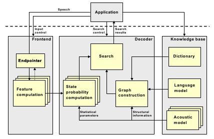
The Sphinx-4 architecture has been designed with a high degree of modularity. Figure 1 shows the overall architecture of the system. Even within each module shown in Figure 1, the code is extremely modular with easily replaceable functions. [10]

Sphinx4 architecture

Figure 1: Architecture of the Sphinx-4 system. The main blocks are Frontend, Decoder and Knowledge base. Except for the blocks within the KB, all other blocks are independently replaceable software modules written in Java. Stacked blocks indicate multiple types which can be used simultaneously

3. Initial Implementation Considerations
Regarding the CRF models, there is already a java implementation [11] which is based on the original CRF paper by J. Lafferty et al [12].
For the JMM models, there are many different approaches proposed [6], [13], [14] and all of them provide the implementation code (in C++/python) as free software available at [15], [16] and [17] respectively.
Another point regarding the JMM models, is the implementation of Weighted Finite State Transducers in java. Two possible approaches would be to a) either reimplement OpenFST Library [18] in java (it is written in C++) or b) investigate if the classes under the fst package [19] of the MARY Text-to-Speech System [20] can be easily integrated in cmusphinx, or if it can just be the basis for a new WFST implementation in Java.

4. Conclusion – Future work
The modular architecture of Sphinx-4 allows for experimentation in emerging areas of research and gives the ability to researchers to easily replace most of it’s parts.
On a recent paper [21] Jouvet et al. propose the combination of two g2p converters, one based on joint multigram model (JMM) and one on conditional random fields (CRF). They evaluate the g2p conversion in a speech recognition context using French broadcast news data and cmusphinx.
During the Google Summer of Code 2012, I will follow a similar approach as in the above paper in order to evaluate and implement the necessary code for g2p conversion in sphinx-4.
You can follow my progress by subscribing to my project’s blog feeds [22]

References
[1] H. U. Hein, “Automation of the training procedures for neural networks performing multi-lingual grapheme to phoneme conversion”, EUROSPEECH’99, pp. 2087-2090, 1999.
[2] I. Stoianov, L. Stowe, and J. Nerbonne, “Connectionist learning to read aloud and correlation to human data”, Proceedings of the 21st Annual Conference of the Cognitive Science Society. Hillsdale, NJ: Erlbaum, 1999.
[3] J.L. Elman, “Finding structure in time”, Cognitive Science, 14, pp. 213-252, 1990.
[4] W. Daelemans, A. V.D. Bosch, “Language-independent data-oriented grapheme-to-phoneme conversion”, Progress in Speech Synthesis, pp. 77–89. New York, USA, 1997.
[5] D. Jouvet, D. Fohr, I. Illina, “Evaluating Grapheme-to-Phoneme Converters in Automatic Speech Recognition Context”, IEE International Conference on Acoustics, 2012.
[6] M. Bisani, H. Ney, “Joint-sequence models for grapheme-to-phoneme conversion”, Speech Communications, vol. 50, no. 5, 2008.
[7] D. Wang, S. King, “Letter-to-sound Pronunciation Prediction Using Conditional Random Fields”, IEEE Signal Processing Letters, vol. 18, no. 2, pp. 122-125, 2011.
[8] I. Illina, D. Fohr & D. Jouvet, “Grapheme-to-Phoneme Conversion using Conditional Random Fields”, in Proc. INTERSPEECH’2011, Florence, Italy, Aug. 2011.
[9] W. Walker, P. Lamere, P. Kwok, B. Raj, R. Singh, E. Gouvea, P. Wolf, and J. Woelfel, “Sphinx-4: A flexible open source framework for speech recognition”, Technical Report SMLI TR2004-0811, Sun Microsystems Inc., 2004.
[10] P. Lamere, P. Kwok, W. Walker, E. Gouvea, R. Singh, B. Raj, and P. Wolf, “Design of the CMU Sphinx-4 decoder”, Proceedings of the 8th European Conference on Speech Communication and Technology, Geneve, Switzerland, pp. 1181–1184, Sept. 2003.
[11] “CRF Project Page”, last accessed: 24/04/2012
[12] J. Lafferty, A. McCallum, F. Pereira, “Conditional Random Fields: Probabilistic Models for Segmenting and Labeling Sequence Data”, Proceedings of the International Conference on Machine Learning (ICML-2001),2001.
[13] “Phonetisaurus g2p tutorial”,  last accessed: 25/04/2012
[14] S. Jiampojamarn, C. Cherry, G. Kondrak, “Joint Processing and Discriminative Training for Letter-to-Phoneme Conversion”, Proceeding of the Annual Meeting of the Association for Computational Linguistics: Human Language Technologies (ACL-08: HLT), pp.905-913, Columbus, OH, June 2008.
[15] “Sequitur G2P, A trainable Grapheme-to-Phoneme converter”, last accessed: 25/04/2012
[16] “phonetisaurus: A WFST-driven Phoneticizer”, last accessed: 25/04/2012
[17] “DirecTL+ : String transduction model”, http://code.google.com/p/directl-p/ last accessed: 25/04/2012
[18] “OpenFST Library”, last accessed: 25/04/2012
[19] “Javadoc for package marytts.fst”,  last accessed: 25/04/2012
[20] “The MARY Text-to-Speech System”, last accessed: 25/04/2012
[21] D. Jouvet, D. Fohr, I. Illina, “Evaluating Grapheme-to-Phoneme Converters in Automatic Speech Recognition Context”, IEE International Conference on Acoustics, 2012
[22] “GSoC 2012: Letter to Phoneme Conversion in CMU Sphinx-4”, Project progress updates.

Implementation of Elman Recurrent Neural Network in WEKA

Foreword

In this article, we will discuss the implementation of the Elman Network or Simple Recurrent Network (SRN) [1],[2] in WEKA. The implementation of Elman NN in WEKA is actually an extension to the already implemented Multilayer Perceptron (MLP) algorithm [3], so we first study MLP and it’s training algorithm, continuing with the study of Elman NN and its implementation in WEKA based on our previous article on extending WEKA [4].

1. Feedfordward Neural Networks: the Multilayer Perceptron (MLP)

In a feedforward network there is no feedback of the output of a neuron as input to another neuron in which it depends. For a given input \mathbf{x} all the required calculations in order to compute the network’s output take place in the same direction: from input to output neurons [5].

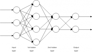
A Multilayer Perceptron (MLP) is a feedforward network in which the neurons are organized in layers. An example of an MLP network is shown in Figure 1. The main characteristic of this type of networks is that there are no connections between the neurons on the same layer. There is one input layer, one output and zero or more hidden layers. Usually all connections begin in a neuron on a layer and end to a neuron on the next layer. Finally, the nodes on the input layer do not perform any calculation, but they simply output their inputs. [5]

A Multilayer Perceptron with 2 hidden layers

Figure 1: A Multilayer Perceptron with 2 hidden layers

1.1. Training of MLP networks (error backpropagation algorithm)

The error backpropagation algorithm for the training of MLP networks was introduced at 1986 in a paper by Rumelhart, Hinton and Williams [6].

In this algorithm a set of training examples D = \left\{ {\left( {{\mathbf{x}}^n ,{\mathbf{t}}^n } \right)} \right\},n = 1,2,..,N are presented to the network, where {\mathbf{x}}^n = \left( {x_{n1} ,.. ,x_{nd} } \right)^T \in \mathbb{R}^d is the input vector and {\mathbf{t}}^n = \left( {t_{n1} ,..,t_{np} } \right)^T \in \mathbb{R}^p is the target output. The network computes its output {\mathbf{o}}\left( {{\mathbf{x}}^n ;{\mathbf{w}}} \right), where {\mathbf{x}}^n is the input vector and {\mathbf{w}} = \left( {w_1 ,..,w_L } \right)^T the vector containing all weights and biases of the network. [5]

We can now define the square of error function [5] as follows:

E({\mathbf{w}}) = \frac{1} {2}\sum\limits_{n = 1}^N {\left\| {{\mathbf{t}}^n - {\mathbf{o}}\left( {{\mathbf{x}}^n ;{\mathbf{w}}} \right)} \right\|^2 } = \frac{1} {2}\sum\limits_{n = 1}^N {\sum\limits_{m = 1}^p {\left( {t_{nm} - o_m \left( {{\mathbf{x}}^n ;{\mathbf{w}}} \right)} \right)^2 } } (1)

which is a sum of square errors per example \left( {{\mathbf{x}}^n ,{\mathbf{t}}^n } \right) and thus is bounded from below by 0, which occurs in case of perfect training. With E^n \left( {\mathbf{w}} \right) is represented the square error per example \left( {{\mathbf{x}}^n ,{\mathbf{t}}^n } \right), and so:

E\left( {\mathbf{w}} \right) = \sum\limits_{n = 1}^N {E^n \left( {\mathbf{w}} \right)} ,E^n \left( {\mathbf{w}} \right) = \frac{1} {2}\left\| {{\mathbf{t}}^n - {\mathbf{o}}\left( {{\mathbf{x}}^n ;{\mathbf{w}}} \right)} \right\|^2 = \frac{1} {2}\sum\limits_{m = 1}^p {\left( {t_{nm} - o_m \left( {{\mathbf{x}}^n ;{\mathbf{w}}} \right)} \right)^2 } (2)

MLP’s training is implemented by updating the weight vector \mathbf{w} in order to minimize the square error E\left( {\mathbf{w}} \right) and it is actually an application of the gradient descent method which starts from an initial weight vector \mathbf{w}(0), and for every repetition k computes the weight vector difference \Delta\mathbf{w}(k) in a way that it moves with small steps to the direction for which the function E\left( {\mathbf{w}} \right) has the greatest rate of decrease. [5]

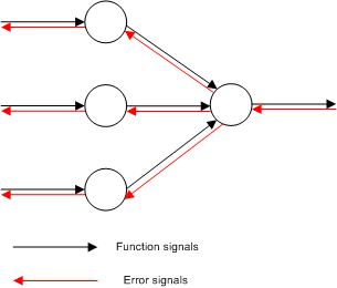
The training is a two-pass transmission through the layers of the networks: a forward propagation and a back propagation as it is depicted in Figure 2. [1]

The directions of two basic signal flows in a multilayer  perceptron.

Figure 2: The directions of two basic signal flows in a multilayer perceptron.

During the forward pass, the output values for all network’s nodes are calculated and stored. These values are also called function signals, their directions are from input to output and at the end is produced a set of outputs {\mathbf{o}}_i ,i = 1,2,..,p which are the network’s output vector. This output vector is then compared with the target output vector {\mathbf{t}}_i ,i = 1,2,..,p and the error signal is produced for the output neurons. That signal is propagated to the opposite direction and the errors for all hidden neurons are calculated. [5]

In order to describe the calculations that take place during the training of the MLP network, we need to define the symbols for the various values. So, we define [5] the i-th neuron on the l-th layer as i^l and thus:

  • u_i^{(l)} the total input of the i^l neuron.
  • y_i^{(l)} the output of the i^l neuron.
  • \delta_i^{(l)} the error of the i^l neuron.
  • w_{i0}^{(l)} the bias of the i^l neuron.
  • g_l the activation function of neurons on the l-th layer.
  • d_l the number of neurons on the l-th layer.
  • w_{ij}^{(l)} the weight of the connection between the neurons j^{l-1} and i^l.

The layers are numbered from the input to output layers and for the input layer l=0. If {\mathbf{x}}^n = \left( {x_1 ,..,x_d } \right)^T is the input vector, then for the input layer’s neurons is y_i^{(0)} = x_i ,x_0 = 1. If q is the output layer, then the network’s output would be o_i \left( {{\mathbf{x}};{\mathbf{w}}} \right) = y_i^{(q)} .

Given an MLP network with d inputs, p outputs and H hidden layers, the input layer is layer 0 and d_0=d, the output layer is layer H+1 and d_{H+1} = p. So, the computation for the output vector {\mathbf{o}}\left( {{\mathbf{x}}^n ;{\mathbf{w}}} \right) = \left( {o_1 ,..,o_p } \right)^T for an input {\mathbf{x}}^n = \left( {x_1 ,..,x_d } \right)^T is as follows: [5]

Forward pass

Input layer

y_i^{(0)} = x_i ,y_0^{(0)} = x_0 = 1 (3)

Hidden and output layers

u_i^{(h)} = \sum\limits_{j = 0}^{d_{h - 1} } {w_{ij}^{(h)} y_j^{(h - 1)} } ,h = 1,..,H + 1,i = ,..,d_h (4)

y_i^{(h)} = g_h \left( {u_i^{(h)} } \right),h = 1,..,H + 1,i = 1,..,d_h ,y_0^{(h)} = 1 (5)

Network’s output

o_i = y_i^{(H + 1)} ,i = 1,..,p (6)

At this point the error back propagation can be applied as follows: [5]

Error backpropagation

Error calculations for the output neurons

\delta _i^{(H + 1)} = g'_{H + 1} \left( {u_i^{(H + 1)} } \right)\frac{{\partial E^n }}{{\partial o_i }},i = 1,..,p (7)

Backpropagation of the errors to the first hidden layer’s neurons

\delta _i^{(h)} = g'_h \left( {u_i^{(h)} } \right)\sum\limits_{j = 1}^{d_{h + 1} } {w_{ij}^{(h + 1)} \delta _j^{(h + 1)} ,h = H,..,1,i = 1,..,d_h } (8)

Calculation of the error’s E^n partial derivatives of the weights

\frac{{\partial E^n }} {{\partial w_{ij}^{(h)} }} = \delta _i^{(h)} y_j^{(h - 1)} (9)

In case that E^n is the square error per example, then, according to the equation (2), equation (8) can be written as:

\delta _i^{(h)} = y_i^{(h)} \left( {1 - y_i^{(h)} } \right)\sum\limits_{j = 1}^{d_{h + 1} } {w_{ij}^{(h + 1)} \delta _j^{(h + 1)} } (10)

and it is not necessary to store the u_i values during the forward pass. This is true also for the output layer’s neurons. So, if their activation function is the logistic, then:

\delta _i^{(H + 1)} = - o_i \left( {1 - o_i } \right)\left( {t_{ni} - o_i } \right) (11)

and if it is linear:

\delta _i^{(H + 1)} = - \left( {t_{ni} - o_i } \right) (12)

The above descriptions can be summarized to the following algorithm:

MLP training algorithm by minimizing the training error

  1. Intialize the weigth vector \mathbf{w}(0) with random values in (1,1), the learning rate \eta, the repetitions counter (\kappa=0) and the epochs counter (k=0).
  2. Let \mathbf{w}(\kappa) the network’s weight vector in the begining of epoch \kappa
    1. Start of epoch k. Store the current values of the weight vector {\mathbf{w}}_{old}=\mathbf{w}(\kappa)
    2. For n=1,2,..,N
      1. Select the training example ({\mathbf{x}}^n,{\mathbf{t}}^n) and aplly the error backpropagation in order to compute the partial derivatives \frac{{\partial E^n }}{{\partial w_i }}
      2. Update the weights
        w_i (\kappa + 1) = w_i (\kappa ) - \eta\frac{{\partial E^n }}{{\partial w_i }} (13)
      3. \kappa = \kappa +1
    3. End of epoch k Termination check. If true, terminate.
  3. k=k+1. Go to step 2.

In equation 13 can be added an extra quantity as in equation 14 below:

w_i (\kappa + 1) = w_i (\kappa ) + \alpha \Delta w_i (\kappa - 1) - n\frac{{\partial E^n }}{{\partial w_i }} (14)

This quantity is called momentum term and the constant \alpha momentum constant. Momentum introduces to the network a kind of memory related to the previous values of \Delta w_i. So we can achieve a stabilizing effect and prevent the phenomenon of oscillations around the value of the minimum error. [5]

2. Recurrent Neural Networks: the Elman Network

The error backpropagation algorithm can be used to solve a wide range of problems. Feedforward networks, however, can only achieve a static mapping of the input space to the output space. In order to be able to model dynamic systems such as the human’s brain, we need to develop a network that is able to store internal states. [7]

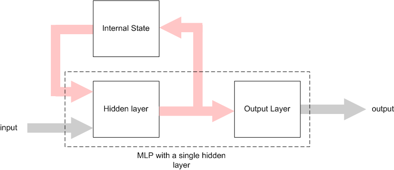
These types of networks are called Recurrent Neural Networks (RNN) and their main characteristic is the internal feedback or time-delayed connections. [7] An architecture of RNN is the Simple Recurrent Network (SRN) or Elman Network (Figure 3). [1] [8]

Architecture of an Elman Network

Figure 3: Architecture of an Elman Network

As we can see from the above figure, an Elman network is an MLP with a single hidden layer and in addirion it contains connections from the hidden layer’s neurons to the context units. The context units store the output values from the hidden neurons in a time unit and these values are fed as additional inputs to the hidden neurons in the next time unit. [1]

Assuming that we have a sequence of input vectors and a clock to synchronize the inputs, then it will take place the following process: The context units are initialized at 0.5. In a given time t the first input vector is presented to the network and with the context units represent the input for the hidden nodes. Following that, the hidden nodes’ outputs are calculated and their values act as an input for the output nodes, and the network’s output is calculated. Finally the hidden nodes’ outputs are also stored to the context units and the procedure is repeated for time t=t+1. [8]

2.1. Training of Elman networks

During the training procedure of an Elman network, similar to the case of an MLP training, the network’s output is compared with the target output and the square error is used to update the network’s weights according to the error backpropagation algorithm [6] with the exception that the values of recurrent connections’ weights are constant to 1.0 [8].

If {\mathbf{x}}^n is the vector produced by the union of input and context vectors, then the training algorithm for an Elman network is very similar to the algorithm for an MLP network training:

Elman training algorithm

  1. Intialize the weigth vector \mathbf{w}(0) with random values in (1,1), the learning rate \eta, the repetitions counter (\kappa=0) and the epochs counter (k=0). Initialize the context nodes at 0.5.
  2. Let \mathbf{w}(\kappa) the network’s weight vector in the begining of epoch \kappa
    1. Start of epoch k. Store the current values of the weight vector {\mathbf{w}}_{old}=\mathbf{w}(\kappa)
    2. For n=1,2,..,N
      1. Select the training example ({\mathbf{x}}^n,{\mathbf{t}}^n) and aplly the error backpropagation in order to compute the partial derivatives \frac{{\partial E^n }}{{\partial w_i }}
      2. Update the weights
        w_i (\kappa + 1) = w_i (\kappa ) - \eta\frac{{\partial E^n }}{{\partial w_i }} (13)
      3. Copy the hidden nodes’ values to the the context units.
      4. \kappa = \kappa +1
    3. End of epoch k Termination check. If true, terminate.
  3. k=k+1. Go to step 2.

3. Implementation of Elman network in WEKA

Elman network implementation is based in the MLP algorithm (already existend in WEKA), which was sligthly modified in some parts like it’s general architecture and the initialization phase. The training algorithm remained the same with the addition of a step which copies the values of the hidden nodes to the context units.

Elman neural network - Parameters in WEKA.

Figure 4: Elman neural network – Parameters in WEKA.

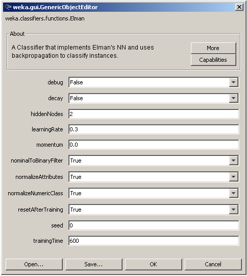
The algorithm’s parameters that can be modified by the user, as shown in Figure 4. above, training parameters such as the learning rate \eta (learningRate), the momentum constant \alpha (momentum) and the number of training epochs k (trainingTime), architectural parameters such as the number of hidden nodes, an option to normalize the input vector (normalizeAttributes) and the output numeric value (normalizeNumericClass) and also an option to transform nominal input values to binary (nominalToBinaryFilter). The seed parameter is used to initialize a random number generator for the initial randomization of the network’s weights. Finally, the parameter resetAfterTraining defines if the internal state will be reseted or not after the training is complete.

4. Conclusions

In this article, we saw the differences between a common type of feedforwand network (MLP) and a recurrent network (Elman or SRN). We saw also how the elman neural network can be implemented in WEKA by modifying the code of the existing MLP network. The source code of the current Elman implementation for WEKA can be found at Elman.zip is not included as an official package in WEKA as it cannot be integrated well in WEKA due to the lack of support for classifiers that contain an internal state. On the other hand it can be used in custom java code and it is already been used with sucess in my own BSc Thesis [9].

References

[1] S. Haykin, “Neural Networks and Learning Machines”, 3rd Edition, Pearson Education, 2008.

[2] J. Elman, “Finding structure in time”, Cognitive Science, 1990, vol. 14, pp. 179-211.

[3] I. H. Witten, E. Frank, “Data Mining – Practical Machine Learning Tools and Techniques”, 2nd Edition, Elsevier, 2005.

[4] J. Salatas, “Extending Weka”, ICT Research Blog, August 2011.

[5] Α. Λύκας, “Τεχνητά Νευρωνικά Δίκτυα – Εφαρμογές”, Τεχνητή Νοημοσύνη Εφαρμογές, Τόμος Β, Ελληνικό Ανοικτό Πανεπιστήμιο, 2008.

[6] D. Rumelhart, G. Hinton, R. Williams. “Learning Internal Representations by Error Propagation”, Parallel Distributed Processing, MIT Press, 1986, pp.918-362.

[7] K. Doya, “Recurrent Networks: Learning Algorithms”, The Handbook of Brain Theory and Neural Networks, 2nd Edition, MIT Press, 2003. pp. 955-960.

[8] J. Elman, “Finding structure in time”, Cognitive Science, 1990, vol. 14, pp. 179-211.

[9] J. Salatas, “Implementation of Artificial Neural Networks and Applications in Foreign Exchange Time Series Analysis and Forecasting”, Hellenic Open University, May 2011.