Foreword

In a previous article, we shown that by using WEKA a researcher can easily implement her own algorithms without other technical concernings like binding an algorithm with a GUI or even loading the data from a file/database, as these tasks and many others are handled transparently by the WEKA framework. [1]

In this article we will study Competitive Learning Networks and more especially the Learning Vector Quantization and Self-Organizing Maps architectures. Finally we will describe the implementation of these networks for WEKA. [2]

1. Competitive Learning Networks

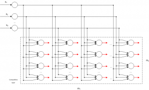
Competitive Learning is usually implemented with Neural Networks that contain a hidden layer which is commonly called as “competitive layer” (see Figure 1). Every competitive neuron $i$ is described by a vector of weights ${\mathbf{w}}_i = \left( {w_{i1} ,..,w_{id} } \right)^T ,i = 1,..,M$ and calculates the similarity measure between the input data ${\mathbf{x}}^n = \left( {x_{n1} ,..,x_{nd} } \right)^T \in \mathbb{R}^d$ and the weight vector ${\mathbf{w}}_i$ . [3]

Figure 1: Competitive neural network architecture

For every input vector, the competitive neurons “compete” each other for the winner neuron, which its weight vector has the greatest similarity for that particular input vector. The winner neuron m sets its output $o_i = 1$ and all the other competitive neuron set their output $o_i = 0 , i = 1,..,M, i \ne m$ . [3]

Usually as similarity measure is used a function of the inverse of Euclidean distance $\left\| {{\mathbf{x}} - {\mathbf{w}}_i } \right\|$ between the input vector ${\mathbf{x}}^n$ and the weight vector ${\mathbf{w}}_i$ . [3]

1.1. Learning Vector Quantization (LVQ)

The algorithm for a Learning Vector Quantization can be easily implemented by utilizing a neural network with a competive layer containing a number of competitive neurons equal with the number of clusters. Every competive neuron i corresponds to a cluster and its weight vector ${\mathbf{w}}_i = \left( {w_{i1} ,..,w_{id} } \right)^T ,i = 1,..,M$ corresponds to centroid of the cluster $i$ . [3]

The algorithm is repetitive and requires the initialization of the networks weight vectors ${\mathbf{w}}_i$ . In each repetition or epoch a vector ${\mathbf{x}}^n$ is presented as input to the network, the distances from each centroid ${\mathbf{w}}_i$ are calcualeted and finally the winner neuron $m$ with the the minimum value of Euclidean distance $d^2 \left( {{\mathbf{x}}^n ,{\mathbf{w}}_m } \right) = \sum_{j = 1}^{d} {(x_j - w_{ij})^2}$ is selected. The final step is to update the weight vectors by “moving” the winner’s neuron centroid $w_m$ “closer” to the input vector ${\mathbf{x}}^n$ . The amount of the “moving” depends on a η parameter (learning rate).

LVQ clustering algorithm

Define the number of clusters $M$ .
Initialize the $M$ centroids ${\mathbf{w}}_i (0),i = 1,..,M$ .
Initialize learning rate $\eta$ , epochs counter $k=0$ and repetitions counter $\kappa = 0$ .
For every epoch do the following steps for
- Set vector $\mathbf{x}^n$ as the Neural Network’s input.
- Select the winner neuron $m$ .
- Update the weight vector for the winner neuron
  $w_{ij} (\kappa + 1) = \left\{ { \begin{array}{ll} {w_{ij} (\kappa )} & {i \ne m} \\ {w_{ij} (\kappa ) + \eta \left( {x_{nj} - w_{ij} (\kappa )} \right)} & i = m \end{array} } , \begin{array}{l} i = 1,..,M \\ j = 1,..,d \end{array} \right.$
- $\kappa = \kappa + 1$ .
Check for termination. If not set $k = k + 1$ and return to step 4.

1.2. Self-Organizing Maps SOM

The Self-Organizing Maps (SOM) is another very common competitive learning alrgorithm that was introduced by Τ. Kohonen [4] in an attempt to model a self-organization process human’s brain.

A SOM network consists of the input layer and a layer containing the competitive neurons which are laid out in a 2 dimensional lattice (see Figure 2) [5]. Each of these neurons are is described by a vector of weights ${\mathbf{w}}_i = \left( {w_{i1} ,..,w_{id} } \right)^T$ . When an input vector $\mathbf{x} = \left( {x_1 ,..,x_d} \right)$ is presented to the network, the lattice’s neurons compete and the winner $m$ is seletcted with its weight vector ${\mathbf{w}}_m$ having the most similarity with $\mathbf{x}$ . So, one can argue that a SOM network is a mapping function of a d-dimensional input $\mathbf{x}$ to a 2-dimensional lattice ${\mathbf{r}}_m = \left( {z_{m1} ,z_{m2} } \right) ^T$ . [3]

Figure 2: A SOM network with d inputs and a 2d lattice m1 x m2

1.2.1. SOM’s Training Algorithm

The algorithm starts by initializing the weights vectors ${\mathbf{w}}_i = \left( {w_{i1} ,..,w_{id} } \right)^T$ to small random values produced by a random number generator. After that step, there three main stages, which can be summarized as follows [3], [5]

Competition: For every training example ${\mathbf{x}}^n$ the lattice’s neurons calculate the value of the similarity function οι νευρώνες. The neuron with the greater similarity becomes the winner neuron.
For the similarity function is usually used the Euclidean distance between the input vector ${\mathbf{x}}^n = \left( {x_1 ,..,x_d} \right)^T$ and the weight vectors ${\mathbf{w}}_i = \left( {w_{i1} ,..,w_{id} } \right)^T$ for each competitive neuron.
Cooperation: The winner neuron defines in the lattice the topological neighbor. The neurons which belong to that neighbor will all update their weights for the given input.
A basic question has to do with the topological neighbor’s definition. Let’s define as the topological neighbor, with its center on the wining neuron . The topological neighbor consists of a set of neurons, and is a random neuron in this set. We also define as the distance between the wining neuron and the neuron . We can now assume that the topological neighbor is a function of that satisfies two criteria: [5]
- Is symmetrical to the point that the function has its largest value and for which is $d_{j,i} = 0$ , or in other words to the winner neuron’s point.
- The function’s amplitude decreases monotonically, as the distance $d_{j,i}$ from the winner neuron increases, approaching zero when the distance $d_{j,i}$ tends to infinity.

A function that satisfies the above criteria is the Gauss function:

$h_{j,i} \left( {\mathbf{x}} \right) = \exp \left( { - \frac{{d_{j,i}^2 }} {{2\sigma ^2 }}} \right)$ (1)

where $\sigma$ is the effective width of the topological neighbor, which determines the extend to which each neuron in the topological neighbor participate in the learning process. This parameter is decreased exponentially in each epoch $n$ according to the following formula: [5]

$\sigma \left( n \right) = \sigma _0 \exp \left( { - \frac{n}{{\tau _1 }}} \right),n = 0,1,2,..$ (2)

where $\sigma _0$ is the effective width’s initial value and $\tau _1$ a constant chosen by the network’s designer. [5]

Synaptic Adaption: In this last stage take place the weight vector adjustments for the neurons in the lattice, as per the following equation: [5]

$\Delta w_j = \eta h_{j,i({\mathbf{x}})}\left( {{\mathbf{x}} - {\mathbf{w}}_j } \right), \left\{ \begin{array} {l} i:\text{winner neuron} \\ j:\text{neuron in } i \text{s neighbor} \end{array} \right.$ (3)

Finally, given a weights vector ${\mathbf{w}}_{j}(n)$ for epoch $n$ , one can easily calculate the new vector for epoch $n+1$ using the equation: [5]

$w_j (n + 1) = w_j (n) + \eta (n)h_{j,i({\mathbf{x}})} \left( n \right)\left( {{\mathbf{x}}(n) - {\mathbf{w}}_j (n)} \right)$ (4)

As we can see in the last formula, the learning rate $\eta (n)$ is also time (epoch) depended. To be more specific, the learning rate should be initialized at a value $\eta_0$ and decrease exponentially with the increase of time (epoch) counter $n$ : [5]

$\eta \left( n \right) = \eta _0 \exp \left( { - \frac{n} {{\tau _2 }}} \right),n = 0,1,2,..$ (5)

where $\tau_2$ is another constant chosen by the network’s designer.

The procedures described above may further be divided into two phases: [4]

Ordering phase, is the first phase, during which takes place the topological arrangement of the weights vectors of neurons in the competitive level. In this phase the learning rate $\eta (n)$ should start from a value near 0.1 and decrease gradually down to 0.01. These values can be produced by assigning in equation (5) the following values: [5]

$\eta_0 = 0.1, \tau_2 = 1000$ (6)

Furthermore, the topological neighbor function $h_{j,i} (n)$ should initially contain almost all neurons in the lattice with the center being the winner neuron and gradually shrink to contain a few neurons or the winner neuron only. In case of a 2-dimensional lattice, we can set the initial effective width’s value $\sigma_0$ equal with the lattice’s “radius” and also set the value of $\tau_1$ in equation (2) equal to: [5]

$\tau _1 = \frac{1000}{\log \sigma _0 }$ (7)

Convergence phase, in which the weights get their final values, by further adjusting to the input data. In this phase the number of repetitions (epochs) depends on the input vectors’ dimensions an as a rule of thumb should be at minimum 500 times the number of competitive neurons. The learning rate $\eta (n)$ should take values near 0.01 and, finally, the topological neighbor function $h_{j,i} (n)$ should include only the nearest neurons to the winning neuron but also can end up including only the winning neuron. [5]

By summarizing the above descriptions, SOM’s learning algorithm is as follows [3]

SOM training algorithm (continuous neighborhood)

Calculate the number of neurons in the competitive layer $M = m_1*m_2$
Initialize the $M$ centroids ${\mathbf{w}}_i(0), i=1,..,M$
Initialize learning rate $\eta(0)$ , parameter $\sigma(0)$ , epochs counter $k=0$ and repetitions counter $\kappa=0$ .
For each epoch do the following steps for
- Set vector ${\mathbf{x}}^n$ as the Neural Network’s input.
- Select the winner neuron $m$ .
- Update the weight vectors for all neurons in the neighbor of the winning neuron:
  $h_{m,i} \left( \kappa \right) = \exp \left( { - \frac{{\left\| {{\mathbf{r}}_m - {\mathbf{r}}_i } \right\|^2 }}{{2\sigma ^2 (\kappa )}}} \right),i = 1,..,M$ (8)
  $w_{ij} (\kappa + 1) = w_{ij} (\kappa ) + \eta (\kappa )h_{m,i} \left( \kappa \right)\left( {x_{nj} - w_{ij} (\kappa )} \right),j = 1,..,d$ (9)
- $\kappa = \kappa + 1$
Gradually decrease the learning rate $\eta (k)$
Gradually decrease the effective width $\sigma (k)$
Check for termination. If not set $k = k + 1$ and return to step 4.

2. Implementation of LVQ and SOM networks in WEKA

2.1. SOM Network

The SOM Network was implemented according to the description in paragraph 1.3. For the calculation of the learning rate’s and effective width’s values in the ordering phase, in each epoch where used the formulas (5) and (2) accordingly with parameter values

$\tau_2 = \frac{n_o}{\ln (100 \cdot \eta_0)}$

and

$\tau_1 = \frac{n_o}{\ln \sigma_0}$

where $n_o$ the number of epoca in the ordering phase, $\eta_0$ the initial learning rate and $\sigma_0$ the initial effective width which is given by the following formula

$\sigma _0 = \sqrt {w^2 + h^2 }$

where $w$ and $h$ the width and height accordingly of the 2-dimensional lattice.

In the convergence phase the learning rate’s and effective width’s values remain constant equal to 0.01 and 0.0001 accordingly.

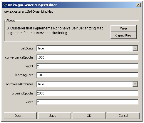
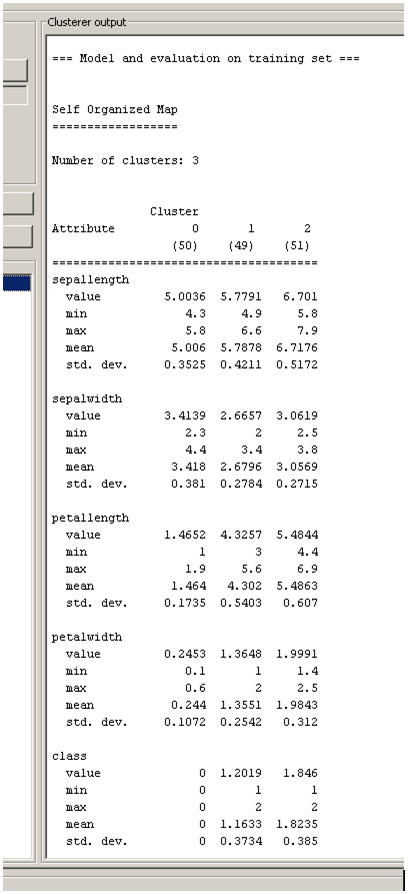
The user adjusted parameters are shown in Figure 3. The 2 dimensions of the lattice can be set via the height and width parameters, the number of epochs for each phase via the orderingEpochs and convergenceEpochs parameters and the initial learning rate via the learningRate parameter. There is also an option for input normalization (normalizeAttributes) and finally the calcStats option for the calculation of some useful information about each cluster as shown in Figure 4.

Figure 3: Self-Organizing Map’s parameters in WEKA

Figure 4: Clustering statistics in 3 clusters for iris.arff dataset dataset using SOM algorithm

2.2. LVQ Network

The LVQ Network was implemented according to the description in paragraph 1.2 based on the source code of SOM network as it was described previously. The code needed only some minor changes with the most important of them being the update of only the winning neuron’s weights. Furthermore, the learning rate remains constant during all training epochs and finally the competitive layer has only one dimension. In other words, the number of clusters is defined with one parameter in contrast with the SOM’s width x height parameters.

Figure 5: LVQ’s Parameters in WEKA

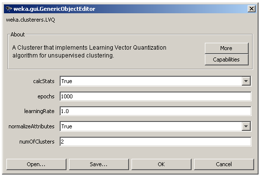
The user adjusted parameters are shown in Figure 5 and contain the learning rate (learningRate), the number of clusters (numOfClusters) and the number of epochs (epochs). Finally, the user can still choose to normalize the input data and to enable the statistics calculations as in the case of SOM.

3. Conclusion

In this article were described two common competitive algorithms. Based on these descriptions the algorithms were implemented for the WEKA framework and they are distributed as official packages that can be installed automatically through WEKA’s package management system [6].

References

[1] J. Salatas, “Extending Weka”, ICT Research Blog, August 2011.

[2] “WEKA Neural Networks Algorithms”
last accessed: 23/08/2011

[3] Α. Λύκας, “Τεχνητά Νευρωνικά Δίκτυα – Εφαρμογές”, Τεχνητή Νοημοσύνη Εφαρμογές, Τόμος Β, Ελληνικό Ανοικτό Πανεπιστήμιο, 2008.

[4] T. Kohonen, “Self-Organization and Associative memory”, 3rd Edition, Springer 1989.

[5] S. Haykin, “Neural Networks and Learning Machines”, 3rd Edition, Pearson Education, 2008.

[6] “How do I use the package manager?”, Weka wiki
last accessed: 24/08/2011

19 thoughts on “Implementation of Competitive Learning Networks for WEKA”

upi 11/07/2011

I am interested in the Implementation of SOM networks in WEKA. The article is nice and clear. After building SOM model in WEKA, I do not understand how to evaluate the SOM model in WEKA so that we can see the effect of different settings; different values of learning rate, width and height.

Reply ↓
1. John Salatas Post author11/07/2011
  
  Assuming that you already have installed SOM package in WEKA you can find additiomal information on how to train and evaluate it (and any other clusterer) at http://www.ibm.com/developerworks/opensource/library/os-weka2/index.html?ca=drs-
  
  Reply ↓
  1. upi 11/07/2011
    
    thank you for the info.
    I found out that I can wrap the algorithm inside MakeDensityBasedClusterer so that I can view the loglikelihood of the trained model.
    
    Reply ↓
    1. John Salatas Post author11/07/2011
      
      Exactly. Actually, you can use it anywhere that you can you may use Clusterers in general.
      
      Reply ↓
      1. upi 11/09/2011
        
        I have a question related to the output. On the output, there is a value that is really similar to the mean. What does it represent?
        
        thank you
John Salatas Post author11/10/2011

What do you mean by “output”?

Reply ↓
1. upi 11/10/2011
  
  I mean the value mentioned on the result buffer output. for example (on article –> Figure 4: Clustering statistics in 3 clusters for iris.arff dataset dataset using SOM algorithm)
  
  sepallength cluster0 cluster1
  value 5.003 5.7791
  min 4.3 4.9
  max 5.8 6.6
  mean 5.006 5.7878
  std.dev 0.3525 0.4211
  
  what does ‘value’ mean on the result above?
  
  Reply ↓
  1. John Salatas Post author11/10/2011
    
    The min, max, mean and st. dev. values are the corresponding statistical values (minimum. maximum, mean and standard deviation) of all samples assigned in that cluster.
    Hope this helps.
    
    Reply ↓
    1. upi 11/11/2011
      
      in the article (Figure 4: Clustering statistics in 3 clusters for iris.arff dataset dataset using SOM algorithm), there are 5 statistic measures. I can understand the min, max, mean and standard dev. Before those 4 statistics, there is another measure called ‘value’. what does it correspond to?
      
      Reply ↓
      1. John Salatas Post author11/11/2011
        
        This is the centroid’s value for the corresponding dimension.
      2. upi 11/11/2011
        
        thank you very much 🙂
        I really appreciate your help.
      3. John Salatas Post author11/19/2011
        
        you ‘re welcome! 🙂
ptp 02/13/2012

I just installed version 3.7.5 of Weka on Windows XP, and installed SelfOrganizingMap and LVQ via the GUI package manager.

If I start Weka Explorer, choose the iris.arff data file, and on the Cluster the SelfOrganizingMap listed is written using gray text rather than black. Also, after choosing SelfOrganizingMap, the Start button (under IgnoreAttributes) is grayed out, will not respond when clicked, and no output is generated. If I choose LVQ instead, I am able to click the start button and get output.

Could you help me get SelfOrganizingMap to run? Any help is greatly appreciated. Thanks!

Reply ↓
1. John Salatas Post author02/14/2012
  
  I just uploaded a new release (1.0.3) that can handle nominal values which you can download directly at https://sourceforge.net/projects/wekann/files/SelfOrganizingMap/
  
  Please notice that it needs some time in order this new release to appear in the package management.
  
  Thanks for your feedback!
  
  Reply ↓
Kama 06/17/2014

Since the two dimensional lattice is flattened, how do we visualize the cluster assignments to the lattice structure ? So basically want to visualize the two dimensional allocation of neurons.

Also some SOMs give intensity mapping to each cell in the lattice, is it possible and if so how?

Thanks

Reply ↓
Luis 09/21/2015

Hi.
Every time I run the SOM in Weka, the number of clusters is always the height x weight. In your example (2×2) was found 3 clusters, but when I run, I got 4, with the same iris.arff. If I change to 1×3 or 3×1 then I got 3 clusters. I tried with different values and different datasets and the result is always the hxw. Is that right?

Reply ↓
1. John Salatas Post author09/22/2015
  
  Yes, the number of clusters should be h x w. I guess that there can be cases that not all of these have instances assigned.
  
  Reply ↓
Fahad 04/25/2016

Hi

Thanks for such great package. How can I get the distance measure value output for every instance in each cluster? I am looking to find out a measure describing the closeness of an instance with the cluster. Suppose if instance ‘i’ is clustered in cluster ‘C’, then I want to know the distance between instance ‘i’ and centroid of cluster ‘C’.

Reply ↓
1. John Salatas Post author04/25/2016
  
  Have a look at the methods
  clusterInstance(Instance i)
  getClusterInstances()
  getClusters()
  
  In general, you can use these methods (in your own java code) in order to do what you are describing
  
  Reply ↓