Author Archives: John Salatas

Implementation of Competitive Learning Networks for WEKA

Foreword

In a previous article, we shown that by using WEKA a researcher can easily implement her own algorithms without other technical concernings like binding an algorithm with a GUI or even loading the data from a file/database, as these tasks and many others are handled transparently by the WEKA framework. [1]

In this article we will study Competitive Learning Networks and more especially the Learning Vector Quantization and Self-Organizing Maps architectures. Finally we will describe the implementation of these networks for WEKA. [2]

1. Competitive Learning Networks

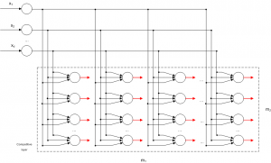
Competitive Learning is usually implemented with Neural Networks that contain a hidden layer which is commonly called as “competitive layer” (see Figure 1). Every competitive neuron $i$ is described by a vector of weights ${\mathbf{w}}_i = \left( {w_{i1} ,..,w_{id} } \right)^T ,i = 1,..,M$ and calculates the similarity measure between the input data ${\mathbf{x}}^n = \left( {x_{n1} ,..,x_{nd} } \right)^T \in \mathbb{R}^d$ and the weight vector ${\mathbf{w}}_i$ . [3]

Figure 1: Competitive neural network architecture

For every input vector, the competitive neurons “compete” each other for the winner neuron, which its weight vector has the greatest similarity for that particular input vector. The winner neuron m sets its output $o_i = 1$ and all the other competitive neuron set their output $o_i = 0 , i = 1,..,M, i \ne m$ . [3]

Usually as similarity measure is used a function of the inverse of Euclidean distance $\left\| {{\mathbf{x}} - {\mathbf{w}}_i } \right\|$ between the input vector ${\mathbf{x}}^n$ and the weight vector ${\mathbf{w}}_i$ . [3]

1.1. Learning Vector Quantization (LVQ)

The algorithm for a Learning Vector Quantization can be easily implemented by utilizing a neural network with a competive layer containing a number of competitive neurons equal with the number of clusters. Every competive neuron i corresponds to a cluster and its weight vector ${\mathbf{w}}_i = \left( {w_{i1} ,..,w_{id} } \right)^T ,i = 1,..,M$ corresponds to centroid of the cluster $i$ . [3]

The algorithm is repetitive and requires the initialization of the networks weight vectors ${\mathbf{w}}_i$ . In each repetition or epoch a vector ${\mathbf{x}}^n$ is presented as input to the network, the distances from each centroid ${\mathbf{w}}_i$ are calcualeted and finally the winner neuron $m$ with the the minimum value of Euclidean distance $d^2 \left( {{\mathbf{x}}^n ,{\mathbf{w}}_m } \right) = \sum_{j = 1}^{d} {(x_j - w_{ij})^2}$ is selected. The final step is to update the weight vectors by “moving” the winner’s neuron centroid $w_m$ “closer” to the input vector ${\mathbf{x}}^n$ . The amount of the “moving” depends on a η parameter (learning rate).

LVQ clustering algorithm

Define the number of clusters $M$ .
Initialize the $M$ centroids ${\mathbf{w}}_i (0),i = 1,..,M$ .
Initialize learning rate $\eta$ , epochs counter $k=0$ and repetitions counter $\kappa = 0$ .
For every epoch do the following steps for
- Set vector $\mathbf{x}^n$ as the Neural Network’s input.
- Select the winner neuron $m$ .
- Update the weight vector for the winner neuron
  $w_{ij} (\kappa + 1) = \left\{ { \begin{array}{ll} {w_{ij} (\kappa )} & {i \ne m} \\ {w_{ij} (\kappa ) + \eta \left( {x_{nj} - w_{ij} (\kappa )} \right)} & i = m \end{array} } , \begin{array}{l} i = 1,..,M \\ j = 1,..,d \end{array} \right.$
- $\kappa = \kappa + 1$ .
Check for termination. If not set $k = k + 1$ and return to step 4.

1.2. Self-Organizing Maps SOM

The Self-Organizing Maps (SOM) is another very common competitive learning alrgorithm that was introduced by Τ. Kohonen [4] in an attempt to model a self-organization process human’s brain.

A SOM network consists of the input layer and a layer containing the competitive neurons which are laid out in a 2 dimensional lattice (see Figure 2) [5]. Each of these neurons are is described by a vector of weights ${\mathbf{w}}_i = \left( {w_{i1} ,..,w_{id} } \right)^T$ . When an input vector $\mathbf{x} = \left( {x_1 ,..,x_d} \right)$ is presented to the network, the lattice’s neurons compete and the winner $m$ is seletcted with its weight vector ${\mathbf{w}}_m$ having the most similarity with $\mathbf{x}$ . So, one can argue that a SOM network is a mapping function of a d-dimensional input $\mathbf{x}$ to a 2-dimensional lattice ${\mathbf{r}}_m = \left( {z_{m1} ,z_{m2} } \right) ^T$ . [3]

Figure 2: A SOM network with d inputs and a 2d lattice m1 x m2

1.2.1. SOM’s Training Algorithm

The algorithm starts by initializing the weights vectors ${\mathbf{w}}_i = \left( {w_{i1} ,..,w_{id} } \right)^T$ to small random values produced by a random number generator. After that step, there three main stages, which can be summarized as follows [3], [5]

Competition: For every training example ${\mathbf{x}}^n$ the lattice’s neurons calculate the value of the similarity function οι νευρώνες. The neuron with the greater similarity becomes the winner neuron.
For the similarity function is usually used the Euclidean distance between the input vector ${\mathbf{x}}^n = \left( {x_1 ,..,x_d} \right)^T$ and the weight vectors ${\mathbf{w}}_i = \left( {w_{i1} ,..,w_{id} } \right)^T$ for each competitive neuron.
Cooperation: The winner neuron defines in the lattice the topological neighbor. The neurons which belong to that neighbor will all update their weights for the given input.
A basic question has to do with the topological neighbor’s definition. Let’s define as the topological neighbor, with its center on the wining neuron . The topological neighbor consists of a set of neurons, and is a random neuron in this set. We also define as the distance between the wining neuron and the neuron . We can now assume that the topological neighbor is a function of that satisfies two criteria: [5]
- Is symmetrical to the point that the function has its largest value and for which is $d_{j,i} = 0$ , or in other words to the winner neuron’s point.
- The function’s amplitude decreases monotonically, as the distance $d_{j,i}$ from the winner neuron increases, approaching zero when the distance $d_{j,i}$ tends to infinity.

A function that satisfies the above criteria is the Gauss function:

$h_{j,i} \left( {\mathbf{x}} \right) = \exp \left( { - \frac{{d_{j,i}^2 }} {{2\sigma ^2 }}} \right)$ (1)

where $\sigma$ is the effective width of the topological neighbor, which determines the extend to which each neuron in the topological neighbor participate in the learning process. This parameter is decreased exponentially in each epoch $n$ according to the following formula: [5]

$\sigma \left( n \right) = \sigma _0 \exp \left( { - \frac{n}{{\tau _1 }}} \right),n = 0,1,2,..$ (2)

where $\sigma _0$ is the effective width’s initial value and $\tau _1$ a constant chosen by the network’s designer. [5]

Synaptic Adaption: In this last stage take place the weight vector adjustments for the neurons in the lattice, as per the following equation: [5]

$\Delta w_j = \eta h_{j,i({\mathbf{x}})}\left( {{\mathbf{x}} - {\mathbf{w}}_j } \right), \left\{ \begin{array} {l} i:\text{winner neuron} \\ j:\text{neuron in } i \text{s neighbor} \end{array} \right.$ (3)

Finally, given a weights vector ${\mathbf{w}}_{j}(n)$ for epoch $n$ , one can easily calculate the new vector for epoch $n+1$ using the equation: [5]

$w_j (n + 1) = w_j (n) + \eta (n)h_{j,i({\mathbf{x}})} \left( n \right)\left( {{\mathbf{x}}(n) - {\mathbf{w}}_j (n)} \right)$ (4)

As we can see in the last formula, the learning rate $\eta (n)$ is also time (epoch) depended. To be more specific, the learning rate should be initialized at a value $\eta_0$ and decrease exponentially with the increase of time (epoch) counter $n$ : [5]

$\eta \left( n \right) = \eta _0 \exp \left( { - \frac{n} {{\tau _2 }}} \right),n = 0,1,2,..$ (5)

where $\tau_2$ is another constant chosen by the network’s designer.

The procedures described above may further be divided into two phases: [4]

Ordering phase, is the first phase, during which takes place the topological arrangement of the weights vectors of neurons in the competitive level. In this phase the learning rate $\eta (n)$ should start from a value near 0.1 and decrease gradually down to 0.01. These values can be produced by assigning in equation (5) the following values: [5]

$\eta_0 = 0.1, \tau_2 = 1000$ (6)

Furthermore, the topological neighbor function $h_{j,i} (n)$ should initially contain almost all neurons in the lattice with the center being the winner neuron and gradually shrink to contain a few neurons or the winner neuron only. In case of a 2-dimensional lattice, we can set the initial effective width’s value $\sigma_0$ equal with the lattice’s “radius” and also set the value of $\tau_1$ in equation (2) equal to: [5]

$\tau _1 = \frac{1000}{\log \sigma _0 }$ (7)

Convergence phase, in which the weights get their final values, by further adjusting to the input data. In this phase the number of repetitions (epochs) depends on the input vectors’ dimensions an as a rule of thumb should be at minimum 500 times the number of competitive neurons. The learning rate $\eta (n)$ should take values near 0.01 and, finally, the topological neighbor function $h_{j,i} (n)$ should include only the nearest neurons to the winning neuron but also can end up including only the winning neuron. [5]

By summarizing the above descriptions, SOM’s learning algorithm is as follows [3]

SOM training algorithm (continuous neighborhood)

Calculate the number of neurons in the competitive layer $M = m_1*m_2$
Initialize the $M$ centroids ${\mathbf{w}}_i(0), i=1,..,M$
Initialize learning rate $\eta(0)$ , parameter $\sigma(0)$ , epochs counter $k=0$ and repetitions counter $\kappa=0$ .
For each epoch do the following steps for
- Set vector ${\mathbf{x}}^n$ as the Neural Network’s input.
- Select the winner neuron $m$ .
- Update the weight vectors for all neurons in the neighbor of the winning neuron:
  $h_{m,i} \left( \kappa \right) = \exp \left( { - \frac{{\left\| {{\mathbf{r}}_m - {\mathbf{r}}_i } \right\|^2 }}{{2\sigma ^2 (\kappa )}}} \right),i = 1,..,M$ (8)
  $w_{ij} (\kappa + 1) = w_{ij} (\kappa ) + \eta (\kappa )h_{m,i} \left( \kappa \right)\left( {x_{nj} - w_{ij} (\kappa )} \right),j = 1,..,d$ (9)
- $\kappa = \kappa + 1$
Gradually decrease the learning rate $\eta (k)$
Gradually decrease the effective width $\sigma (k)$
Check for termination. If not set $k = k + 1$ and return to step 4.

2. Implementation of LVQ and SOM networks in WEKA

2.1. SOM Network

The SOM Network was implemented according to the description in paragraph 1.3. For the calculation of the learning rate’s and effective width’s values in the ordering phase, in each epoch where used the formulas (5) and (2) accordingly with parameter values

$\tau_2 = \frac{n_o}{\ln (100 \cdot \eta_0)}$

and

$\tau_1 = \frac{n_o}{\ln \sigma_0}$

where $n_o$ the number of epoca in the ordering phase, $\eta_0$ the initial learning rate and $\sigma_0$ the initial effective width which is given by the following formula

$\sigma _0 = \sqrt {w^2 + h^2 }$

where $w$ and $h$ the width and height accordingly of the 2-dimensional lattice.

In the convergence phase the learning rate’s and effective width’s values remain constant equal to 0.01 and 0.0001 accordingly.

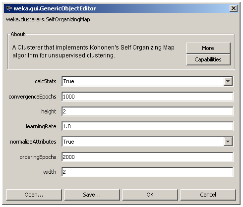
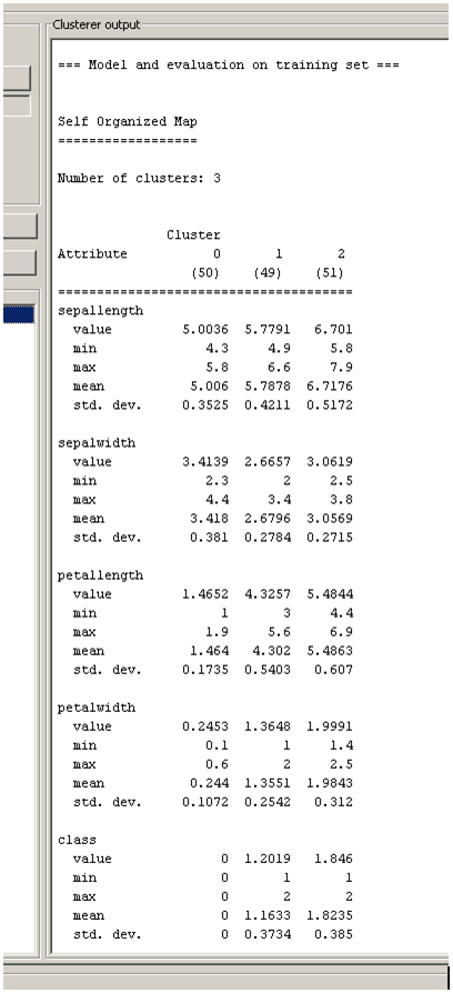
The user adjusted parameters are shown in Figure 3. The 2 dimensions of the lattice can be set via the height and width parameters, the number of epochs for each phase via the orderingEpochs and convergenceEpochs parameters and the initial learning rate via the learningRate parameter. There is also an option for input normalization (normalizeAttributes) and finally the calcStats option for the calculation of some useful information about each cluster as shown in Figure 4.

Figure 3: Self-Organizing Map’s parameters in WEKA

Figure 4: Clustering statistics in 3 clusters for iris.arff dataset dataset using SOM algorithm

2.2. LVQ Network

The LVQ Network was implemented according to the description in paragraph 1.2 based on the source code of SOM network as it was described previously. The code needed only some minor changes with the most important of them being the update of only the winning neuron’s weights. Furthermore, the learning rate remains constant during all training epochs and finally the competitive layer has only one dimension. In other words, the number of clusters is defined with one parameter in contrast with the SOM’s width x height parameters.

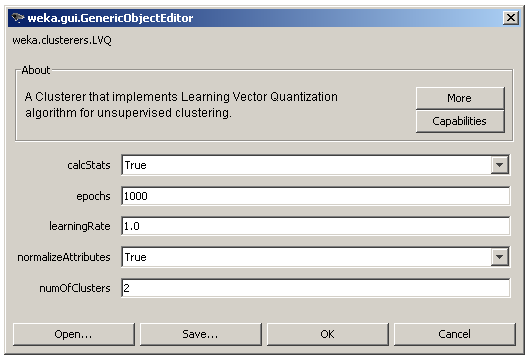
Figure 5: LVQ’s Parameters in WEKA

The user adjusted parameters are shown in Figure 5 and contain the learning rate (learningRate), the number of clusters (numOfClusters) and the number of epochs (epochs). Finally, the user can still choose to normalize the input data and to enable the statistics calculations as in the case of SOM.

3. Conclusion

In this article were described two common competitive algorithms. Based on these descriptions the algorithms were implemented for the WEKA framework and they are distributed as official packages that can be installed automatically through WEKA’s package management system [6].

References

[1] J. Salatas, “Extending Weka”, ICT Research Blog, August 2011.

[2] “WEKA Neural Networks Algorithms”
last accessed: 23/08/2011

[3] Α. Λύκας, “Τεχνητά Νευρωνικά Δίκτυα – Εφαρμογές”, Τεχνητή Νοημοσύνη Εφαρμογές, Τόμος Β, Ελληνικό Ανοικτό Πανεπιστήμιο, 2008.

[4] T. Kohonen, “Self-Organization and Associative memory”, 3rd Edition, Springer 1989.

[5] S. Haykin, “Neural Networks and Learning Machines”, 3rd Edition, Pearson Education, 2008.

[6] “How do I use the package manager?”, Weka wiki
last accessed: 24/08/2011

Extending WEKA

Foreword

This article is part of John’s Salatas BSc. Thesis with subject “Implementation of Artificial Neural Networks and Applications in Foreign Exchange Time Series Analysis and Forecasting” (Greek text) completed at May 2011 under the supervision of Ass. Prof. C. N. Anagnostopoulos (Cultural Technology and Communication Dpt., University of Aegean).

1. Introduction to WEKA

The WEKA environment (Waikato Environment for Knowledge Analysis) [1] was created by the need for an integrated computing environment that would provide to researchers easy access to many machine learning algorithms and also provide a programming environment in which researchers can implement new algorithms without having to consider many programming details. WEKA already has a large number of algorithms and distributed under the license GNU GPL v2. It is developed using the Java programming language and is available at the WEKA’s website.

2. Extending WEKA

WEKA’s Application Programming Interface (API) allows the easy embedding in other java applications as well as extending it with new features that may be either additional machine learning algorithms and tools for data visualization, or even extensions of the Graphical User Interface (GUI) in order to support different workflows, as for example, the Time Series Analysis and Forecasting Environment [2].

The above characteristics are supplemented with the excellent technical support provided by the online user community through the relevant mailing list [3] and the documentation provided through the relevant wiki pages [4].

A good introduction on embedding WEKA in other applications can be found at [5] which describes the most basic and widely used components through a number of examples. The complete documentation (javadoc) of WEKA’s API can be found a [6].

2.1. 3rd Party Tools

Besides WEKA’s source code, in order to implement any extension, one may use a number of external 3rd party programming tools and libraries which are described below. The purpose of these tools is to automate many common programming tasks, such as unit testing or the source code’s management.

2.1.1. Unit Testing – The JUnit Library

For unit testing, WEKA uses the JUnit Library. JUnit is a framework used for the creation of automated test cases and is distributed for free under the License Common Public License v 1.0. A good introduction to the way of writing and organization of these scenarios is available at [7].

2.1.2. Source Code Management – Subversion

WEKA’s source code is also available through a software repository based on Apache Subversion. The Apache Subversion application enables developers to control the modifications to the source code in various stages of the software development cycle, leading to a more efficient collaboration between those involved in the development and thus, to increased productivity, especially in the case of developing a large open source applications, which involves a large number of geographically distributed developers.

Apache Subversion is distributed for free under the Common Public License v 1.0 and a good introduction to this application is available at [8]. Finally, at [9] one can find brief instructions on how to use Apache Subversion with WEKA’s software repository.

2.1.3. Build Scripts – Apache Ant

The build process for a new WEKA extension package requires the Apache Ant build tool which is also distributed for free under the Apache License version 2.0 and a good introduction to this application is available at [10].

2.1.4. Integrated Development Environments (IDE) – Netbeans and Eclipse

The tools described above are usually integrated with other programming tools (i.e. code editors/debuggers) in a single IDE. The two most popular IDE’s for Java development probably are the following:

Netbeans, which is distributed for free under a double license: Common Development and DistributionLicense (CDDL) v1.0 and GNU GPL v2.
Eclipse, which is also distributed for free under the Eclipse Public License (EPL) v. 1.0.

Both of these IDEs can be setup for the development of WEKA’s extensions according to the instructions provided at [11] and [12].

2.2. Implementation of new Classifiers and Clusterers

2.2.1. Implementation of new Classifier

All classifiers in WEKA should implement the interface weka.classifiers.Classifier. WEKA also provides a number of abstract classes that already implement the weka.classifiers.Classifier interface. These abastract classes for version 3.7.3 are described in details in [13]. The most basic of these are AbstractClassifier which already implements several functions and RandomizableClassifier which inherits from AbstractClassifier and implements an additional parameter to initialize (seed) for a random number generator, if required, as in case of classifiers that need ton initialize random weights.

Properties

In order the algorithm’s parameter to be accessible through the WEKA’s Graphic User Interface (GUI), there must be a property definition, in conformance with the JavaBeans conventions [14], as follows [13]:

public void set<PropertyName>(<Type>) checks whether the supplied value is valid and only then updates the corresponding member variable. In any other case it should ignore the value and output a warning in the console or throw an IllegalArgumentException.
public <Type> get<PropertyName>() performs any necessary conversions of the internal value and returns it.
public String <propertyName>TipText() returns the help text that is available through the GUI. Should be the same as on the command-line. Note: everything after the ﬁrst period “.” gets truncated from the tool tip that pops up in the GUI when hovering with the mouse cursor over the ﬁeld in the GenericObjectEditor.

Furthermore the following methods should be implemented in order the algorithm’s parameter to be accessible through the command-line [13]:

public String[] getOptions() which returns a string array of command-line options that resemble the current classiﬁer setup. Supplying this array to the setOptions(String[]) method must result in the same conﬁguration.
public Enumeration listOptions() returns a java.util.Enumeration of weka.core.Option objects. This enumeration is used to display the help on the command-line, hence it needs to return the Option objects of the superclass as well.
public void setOptions(String[] options) which parses the options that the classiﬁer would receive from a command-line invocation. A parameter and argument are always two elements in the string array.

Capabilities

The method public Capabilities getCapabilities() returns meta-information on what type of data the classiﬁer can handle, in regards to attributes and class attributes.

Building the model

The method public void buildClassifier(Instances instances) builds the model from scratch with the provided dataset. Each subsequent call of this method must result in the same model being built. The buildClassifier method also tests whether the supplied data can be handled at all by the classiﬁer, utilizing the capabilities returned by the getCapabilities() method:

public void buildClassifier(Instances data) throws Exception {
    // test data against capabilities
    getCapabilities().testWithFail(data);
    // remove instances with missing class value,
    // but don't modify original data
    data = new Instances(data);
    data.deleteWithMissingClass();
    // actual model generation
    // ...
}

Instance classification

For the classification of an instance one of the following two method should be used [30]:

public double [] distributionForInstance(Instance instance) returns the class probabilities array of the prediction for the given weka.core.Instance object. If your classiﬁer handles nominal class attributes, then you need to override this method.
public double classifyInstance(Instance instance) returns the classiﬁcation or regression for the given weka.core.Instance object. In case of a nominal class attribute, this method returns the index of the class label that got predicted. You do not need to override this method in this case as the weka.classifiers.Classifier superclass already determines the class label index based on the probabilities array that the distributionForInstance(Instance) method returns (it returns the index in the array with the highest probability; in case of ties the ﬁrst one). For numeric class attributes, you need to override this method, as it has to return the regression value predicted by the model.

Other methods

Beside the above methods, there are several other methods which should be or are highly recommended to be implemented for every classifier:

public String toString() which is used for outputting the built model. This is not required, but it is useful for the user to see properties of the model. Decision trees normally ouput the tree, support vector machines the support vectors and rule-based classiﬁers the generated rules.

public static void main(String [] argv) executes the classiﬁer from command-line. If your new algorithm is called MyClassifier, then use the following code as your main method:

/**
* Main method for executing this classifier.
*
* @param args the options, use "-h" to display options
*/
public static void main(String[] args) {
    AbstractClassifier.runClassifier(new MyClassifier(), args);
}

2.2.2. Implementation of new Clusterer

In general the guidelines for implementing a new clusterer are similar to those described above for implementing a new classifier. All clusterers in WEKA should implement the interface weka.clusterers.Clusterer. WEKA also provides a number of abstract classes that already implement the weka.clusterers.Clusterer interface. These abastract classes for version 3.7.3 are described in details in [13]. The most basic of these are AbstractClusterer which already implements several functions and RandomizableClusterer which inherits from AbstractClusterer and implements an additional parameter to initialize (seed) for a random number generator, if required, as in case of clusterers that need ton initialize random weights.

Properties

public void set<PropertyName>(<Type>) checks whether the supplied value is valid and only then updates the corresponding member variable. In any other case it should ignore the value and output a warning in the console or throw an IllegalArgumentException.
public <Type> get<PropertyName>() performs any necessary conversions of the internal value and returns it.
public String <propertyName>TipText() returns the help text that is available through the GUI. Should be the same as on the command-line. Note: everything after the ﬁrst period “.” gets truncated from the tool tip that pops up in the GUI when hovering with the mouse cursor over the ﬁeld in the GenericObjectEditor.

Furthermore the following methods should be implemented in order the algorithm’s parameter to be accessible through the command-line [13]:

public String[] getOptions() which returns a string array of command-line options that resemble the current clusterer setup. Supplying this array to the setOptions(String[]) method must result in the same conﬁguration.
public Enumeration listOptions() returns a java.util.Enumeration of weka.core.Option objects. This enumeration is used to display the help on the command-line, hence it needs to return the Option objects of the superclass as well.
public void setOptions(String[] options) which parses the options that the clusterer would receive from a command-line invocation. A parameter and argument are always two elements in the string array.

Capabilities

The method public Capabilities getCapabilities() returns meta-information on what type of data the clusterer can handle, in regards to attributes and class attributes.

Building the model

The method public void buildClusterer(Instances instances) builds the model from scratch with the provided dataset. Each subsequent call of this method must result in the same model being built. The buildClassifier method also tests whether the supplied data can be handled at all by the clusterer, utilizing the capabilities returned by the getCapabilities() method:

public void buildClusterer(Instances data) throws Exception {
    // test data against capabilities
    getCapabilities().testWithFail(data);
    // actual model generation
    ...
}

Instance clustering

For the clustering of an instance one of the following two method should be used [30]:

public double [] distributionForInstance(Instance instance) returns the cluster membership for this weka.core.Instance object. The membership is a double array containing the probabilities for each cluster.
public double clusterInstance(Instance instance) returns the index of the cluster the provided Instance belongs to.

Other methods

Beside the above methods, there are several other methods which should be or are highly recommended to be implemented for every clusterer:

public String toString() which should output some information on the generated model. Even though this is not required, it is rather useful for the user to get some feedback on the built model.

public static void main(String [] argv) executes the clusterer from command-line. If your new algorithm is called MyClusterer, then use the following code as your main method:

/**
* Main method for executing this clusterer.
*
* @param args the options, use "-h" to display options
*/
public static void main(String[] args) {
    AbstractClusterer.runClusterer(new MyClusterer(), args);
}

Finally, another method that is required to be implemented is the public int numberOfClusters() method which should returns the number of clusters that the model contains, after the model has been generated with the buildClusterer(Instances) method.

2.3. Anatomy of a Package

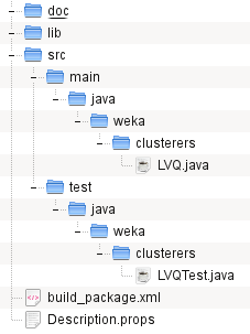
As of version 3.7.2 WEKA can automatically manage extensions that are available as a package. So, the easiest way to distribute an extension is to create a package, which briefly is a zip archive that contains all the resources that are required by the extension. A typical structure for a package is shown in the following image:

The Anatomy of a WEKA’s Package

Under the “src” folder are places all the source code files and under the “test” folder the source code for the unit trsts. The “Description.props” contains the metadata used by the WEKA’s package manager. Finally the file “build_package.xml” contains the package’s build script for the Apache Ant. [15]

3. Conclusion

This article tried to provide a brief description on how to implement new alogoriths in WEKA for data classification and clusterization. We saw that by using WEKA a researcher can easily implement her own algorithms without other technical concernings like binding an algorithm with a GUI or even loading the data from a file/database, as these tasks and many others are handled transparently by the WEKA framework.

References

[1] M. Hall, E. Frank, G. Holmes, B. Pfahringer, P. Reutemann, I. H. Witten, “The WEKA Data Mining Software: An Update”, SIGKDD Explorations, 2009, Volume 11, Issue 1, pp.10-18.

[2] “Time Series Analysis and Forecasting with Weka”, Pentaho Community
last access: 22/08/2011.

[3] “Wekalist – Weka machine learning workbench list”
last access: 22/08/2011.

[4] “Pages”, Weka wiki
last access: 22/08/2011.

[5] “Use WEKA in your Java code”, Weka wiki
last access: 22/08/2011.

[6] “Weka Javadoc”
last access: 22/08/2011.

[7] K. Beck, E. Gamma, “JUnit Cookbook”
last access: 22/08/2011.

[8] B. Collins-Sussman, B. W. Fitzpatrick, C. M. Pilato, “Version Control with
Subversion”, 2008.
last access: 22/08/2011.

[9] “Subversion repository”, Weka wiki
last access: 22/08/2011.

[10] “Apache Ant 1.8.2 Manual”
last access: 22/08/2011.

[11] “Netbeans 6.0”, Weka wiki
last access: 22/08/2011.

[12] “Eclipse 3.4.x”, Weka wiki
last access: 22/08/2011.

[13] R. R. Bouckaert, E. Frank, M. Hall, R. Kirkby, P. Reutemann, A. Seewald, D.
Scuse, “WEKA Manual for Version 3-7-3”, The University of Waikato, 2010.
last access: 22/08/2011.

[14] “JavaBeans Component Design Conventions”, The J2EE Tutorial, Sun Developer Network, 2002.
last access: 22/08/2011.

[15] “How are packages structured for the package management system?”, Weka
wiki
last access: 22/08/2011.