Foreword

In this article, we will discuss the implementation of the Elman Network or Simple Recurrent Network (SRN) [1],[2] in WEKA. The implementation of Elman NN in WEKA is actually an extension to the already implemented Multilayer Perceptron (MLP) algorithm [3], so we first study MLP and it’s training algorithm, continuing with the study of Elman NN and its implementation in WEKA based on our previous article on extending WEKA [4].

1. Feedfordward Neural Networks: the Multilayer Perceptron (MLP)

In a feedforward network there is no feedback of the output of a neuron as input to another neuron in which it depends. For a given input $\mathbf{x}$ all the required calculations in order to compute the network’s output take place in the same direction: from input to output neurons [5].

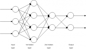
A Multilayer Perceptron (MLP) is a feedforward network in which the neurons are organized in layers. An example of an MLP network is shown in Figure 1. The main characteristic of this type of networks is that there are no connections between the neurons on the same layer. There is one input layer, one output and zero or more hidden layers. Usually all connections begin in a neuron on a layer and end to a neuron on the next layer. Finally, the nodes on the input layer do not perform any calculation, but they simply output their inputs. [5]

Figure 1: A Multilayer Perceptron with 2 hidden layers

1.1. Training of MLP networks (error backpropagation algorithm)

The error backpropagation algorithm for the training of MLP networks was introduced at 1986 in a paper by Rumelhart, Hinton and Williams [6].

In this algorithm a set of training examples $D = \left\{ {\left( {{\mathbf{x}}^n ,{\mathbf{t}}^n } \right)} \right\},n = 1,2,..,N$ are presented to the network, where ${\mathbf{x}}^n = \left( {x_{n1} ,.. ,x_{nd} } \right)^T \in \mathbb{R}^d$ is the input vector and ${\mathbf{t}}^n = \left( {t_{n1} ,..,t_{np} } \right)^T \in \mathbb{R}^p$ is the target output. The network computes its output ${\mathbf{o}}\left( {{\mathbf{x}}^n ;{\mathbf{w}}} \right)$ , where ${\mathbf{x}}^n$ is the input vector and ${\mathbf{w}} = \left( {w_1 ,..,w_L } \right)^T$ the vector containing all weights and biases of the network. [5]

We can now define the square of error function [5] as follows:

$E({\mathbf{w}}) = \frac{1} {2}\sum\limits_{n = 1}^N {\left\| {{\mathbf{t}}^n - {\mathbf{o}}\left( {{\mathbf{x}}^n ;{\mathbf{w}}} \right)} \right\|^2 } = \frac{1} {2}\sum\limits_{n = 1}^N {\sum\limits_{m = 1}^p {\left( {t_{nm} - o_m \left( {{\mathbf{x}}^n ;{\mathbf{w}}} \right)} \right)^2 } }$ (1)

which is a sum of square errors per example $\left( {{\mathbf{x}}^n ,{\mathbf{t}}^n } \right)$ and thus is bounded from below by 0, which occurs in case of perfect training. With $E^n \left( {\mathbf{w}} \right)$ is represented the square error per example $\left( {{\mathbf{x}}^n ,{\mathbf{t}}^n } \right)$ , and so:

$E\left( {\mathbf{w}} \right) = \sum\limits_{n = 1}^N {E^n \left( {\mathbf{w}} \right)} ,E^n \left( {\mathbf{w}} \right) = \frac{1} {2}\left\| {{\mathbf{t}}^n - {\mathbf{o}}\left( {{\mathbf{x}}^n ;{\mathbf{w}}} \right)} \right\|^2 = \frac{1} {2}\sum\limits_{m = 1}^p {\left( {t_{nm} - o_m \left( {{\mathbf{x}}^n ;{\mathbf{w}}} \right)} \right)^2 }$ (2)

MLP’s training is implemented by updating the weight vector $\mathbf{w}$ in order to minimize the square error $E\left( {\mathbf{w}} \right)$ and it is actually an application of the gradient descent method which starts from an initial weight vector $\mathbf{w}(0)$ , and for every repetition $k$ computes the weight vector difference $\Delta\mathbf{w}(k)$ in a way that it moves with small steps to the direction for which the function $E\left( {\mathbf{w}} \right)$ has the greatest rate of decrease. [5]

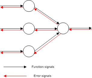
The training is a two-pass transmission through the layers of the networks: a forward propagation and a back propagation as it is depicted in Figure 2. [1]

Figure 2: The directions of two basic signal flows in a multilayer perceptron.

During the forward pass, the output values for all network’s nodes are calculated and stored. These values are also called function signals, their directions are from input to output and at the end is produced a set of outputs ${\mathbf{o}}_i ,i = 1,2,..,p$ which are the network’s output vector. This output vector is then compared with the target output vector ${\mathbf{t}}_i ,i = 1,2,..,p$ and the error signal is produced for the output neurons. That signal is propagated to the opposite direction and the errors for all hidden neurons are calculated. [5]

In order to describe the calculations that take place during the training of the MLP network, we need to define the symbols for the various values. So, we define [5] the $i$ -th neuron on the $l$ -th layer as $i^l$ and thus:

$u_i^{(l)}$ the total input of the $i^l$ neuron.
$y_i^{(l)}$ the output of the $i^l$ neuron.
$\delta_i^{(l)}$ the error of the $i^l$ neuron.
$w_{i0}^{(l)}$ the bias of the $i^l$ neuron.
$g_l$ the activation function of neurons on the $l$ -th layer.
$d_l$ the number of neurons on the $l$ -th layer.
$w_{ij}^{(l)}$ the weight of the connection between the neurons $j^{l-1}$ and $i^l$ .

The layers are numbered from the input to output layers and for the input layer $l=0$ . If ${\mathbf{x}}^n = \left( {x_1 ,..,x_d } \right)^T$ is the input vector, then for the input layer’s neurons is $y_i^{(0)} = x_i ,x_0 = 1$ . If $q$ is the output layer, then the network’s output would be $o_i \left( {{\mathbf{x}};{\mathbf{w}}} \right) = y_i^{(q)}$ .

Given an MLP network with $d$ inputs, $p$ outputs and $H$ hidden layers, the input layer is layer $0$ and $d_0=d$ , the output layer is layer $H+1$ and $d_{H+1} = p$ . So, the computation for the output vector ${\mathbf{o}}\left( {{\mathbf{x}}^n ;{\mathbf{w}}} \right) = \left( {o_1 ,..,o_p } \right)^T$ for an input ${\mathbf{x}}^n = \left( {x_1 ,..,x_d } \right)^T$ is as follows: [5]

Forward pass

Input layer

$y_i^{(0)} = x_i ,y_0^{(0)} = x_0 = 1$ (3)

Hidden and output layers

$u_i^{(h)} = \sum\limits_{j = 0}^{d_{h - 1} } {w_{ij}^{(h)} y_j^{(h - 1)} } ,h = 1,..,H + 1,i = ,..,d_h$ (4)

$y_i^{(h)} = g_h \left( {u_i^{(h)} } \right),h = 1,..,H + 1,i = 1,..,d_h ,y_0^{(h)} = 1$ (5)

Network’s output

$o_i = y_i^{(H + 1)} ,i = 1,..,p$ (6)

At this point the error back propagation can be applied as follows: [5]

Error backpropagation

Error calculations for the output neurons

$\delta _i^{(H + 1)} = g'_{H + 1} \left( {u_i^{(H + 1)} } \right)\frac{{\partial E^n }}{{\partial o_i }},i = 1,..,p$ (7)

Backpropagation of the errors to the first hidden layer’s neurons

$\delta _i^{(h)} = g'_h \left( {u_i^{(h)} } \right)\sum\limits_{j = 1}^{d_{h + 1} } {w_{ij}^{(h + 1)} \delta _j^{(h + 1)} ,h = H,..,1,i = 1,..,d_h }$ (8)

Calculation of the error’s $E^n$ partial derivatives of the weights

$\frac{{\partial E^n }} {{\partial w_{ij}^{(h)} }} = \delta _i^{(h)} y_j^{(h - 1)}$ (9)

In case that $E^n$ is the square error per example, then, according to the equation (2), equation (8) can be written as:

$\delta _i^{(h)} = y_i^{(h)} \left( {1 - y_i^{(h)} } \right)\sum\limits_{j = 1}^{d_{h + 1} } {w_{ij}^{(h + 1)} \delta _j^{(h + 1)} }$ (10)

and it is not necessary to store the $u_i$ values during the forward pass. This is true also for the output layer’s neurons. So, if their activation function is the logistic, then:

$\delta _i^{(H + 1)} = - o_i \left( {1 - o_i } \right)\left( {t_{ni} - o_i } \right)$ (11)

and if it is linear:

$\delta _i^{(H + 1)} = - \left( {t_{ni} - o_i } \right)$ (12)

The above descriptions can be summarized to the following algorithm:

MLP training algorithm by minimizing the training error

Intialize the weigth vector $\mathbf{w}(0)$ with random values in $(1,1)$ , the learning rate $\eta$ , the repetitions counter ( $\kappa=0$ ) and the epochs counter ( $k=0$ ).
Let the network’s weight vector in the begining of epoch
1. Start of epoch $k$ . Store the current values of the weight vector ${\mathbf{w}}_{old}=\mathbf{w}(\kappa)$
2. For
  1. Select the training example $({\mathbf{x}}^n,{\mathbf{t}}^n)$ and aplly the error backpropagation in order to compute the partial derivatives $\frac{{\partial E^n }}{{\partial w_i }}$
  2. Update the weights
    $w_i (\kappa + 1) = w_i (\kappa ) - \eta\frac{{\partial E^n }}{{\partial w_i }}$ (13)
  3. $\kappa = \kappa +1$
3. End of epoch $k$ Termination check. If true, terminate.
$k=k+1$ . Go to step 2.

In equation 13 can be added an extra quantity as in equation 14 below:

$w_i (\kappa + 1) = w_i (\kappa ) + \alpha \Delta w_i (\kappa - 1) - n\frac{{\partial E^n }}{{\partial w_i }}$ (14)

This quantity is called momentum term and the constant $\alpha$ momentum constant. Momentum introduces to the network a kind of memory related to the previous values of $\Delta w_i$ . So we can achieve a stabilizing effect and prevent the phenomenon of oscillations around the value of the minimum error. [5]

2. Recurrent Neural Networks: the Elman Network

The error backpropagation algorithm can be used to solve a wide range of problems. Feedforward networks, however, can only achieve a static mapping of the input space to the output space. In order to be able to model dynamic systems such as the human’s brain, we need to develop a network that is able to store internal states. [7]

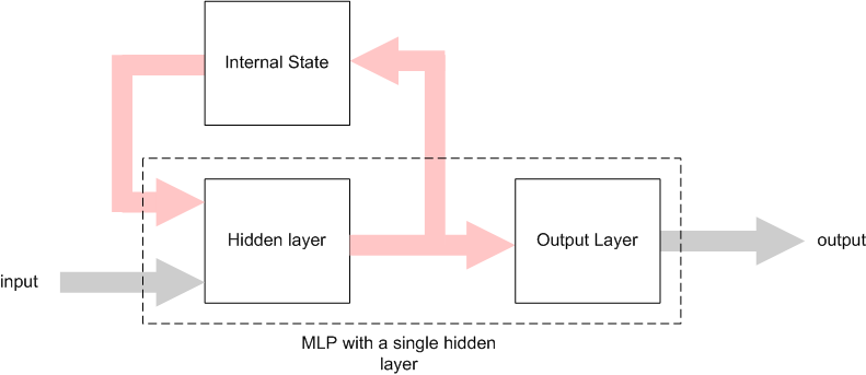
These types of networks are called Recurrent Neural Networks (RNN) and their main characteristic is the internal feedback or time-delayed connections. [7] An architecture of RNN is the Simple Recurrent Network (SRN) or Elman Network (Figure 3). [1] [8]

Figure 3: Architecture of an Elman Network

As we can see from the above figure, an Elman network is an MLP with a single hidden layer and in addirion it contains connections from the hidden layer’s neurons to the context units. The context units store the output values from the hidden neurons in a time unit and these values are fed as additional inputs to the hidden neurons in the next time unit. [1]

Assuming that we have a sequence of input vectors and a clock to synchronize the inputs, then it will take place the following process: The context units are initialized at 0.5. In a given time $t$ the first input vector is presented to the network and with the context units represent the input for the hidden nodes. Following that, the hidden nodes’ outputs are calculated and their values act as an input for the output nodes, and the network’s output is calculated. Finally the hidden nodes’ outputs are also stored to the context units and the procedure is repeated for time $t=t+1$ . [8]

2.1. Training of Elman networks

During the training procedure of an Elman network, similar to the case of an MLP training, the network’s output is compared with the target output and the square error is used to update the network’s weights according to the error backpropagation algorithm [6] with the exception that the values of recurrent connections’ weights are constant to 1.0 [8].

If ${\mathbf{x}}^n$ is the vector produced by the union of input and context vectors, then the training algorithm for an Elman network is very similar to the algorithm for an MLP network training:

Elman training algorithm

Intialize the weigth vector $\mathbf{w}(0)$ with random values in $(1,1)$ , the learning rate $\eta$ , the repetitions counter ( $\kappa=0$ ) and the epochs counter ( $k=0$ ). Initialize the context nodes at 0.5.
Let the network’s weight vector in the begining of epoch
1. Start of epoch $k$ . Store the current values of the weight vector ${\mathbf{w}}_{old}=\mathbf{w}(\kappa)$
2. For
  1. Select the training example $({\mathbf{x}}^n,{\mathbf{t}}^n)$ and aplly the error backpropagation in order to compute the partial derivatives $\frac{{\partial E^n }}{{\partial w_i }}$
  2. Update the weights
    $w_i (\kappa + 1) = w_i (\kappa ) - \eta\frac{{\partial E^n }}{{\partial w_i }}$ (13)
  3. Copy the hidden nodes’ values to the the context units.
  4. $\kappa = \kappa +1$
3. End of epoch $k$ Termination check. If true, terminate.
$k=k+1$ . Go to step 2.

3. Implementation of Elman network in WEKA

Elman network implementation is based in the MLP algorithm (already existend in WEKA), which was sligthly modified in some parts like it’s general architecture and the initialization phase. The training algorithm remained the same with the addition of a step which copies the values of the hidden nodes to the context units.

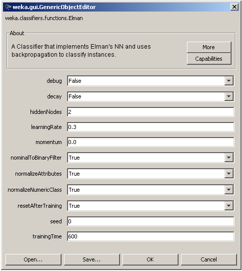
Figure 4: Elman neural network – Parameters in WEKA.

The algorithm’s parameters that can be modified by the user, as shown in Figure 4. above, training parameters such as the learning rate $\eta$ (learningRate), the momentum constant $\alpha$ (momentum) and the number of training epochs $k$ (trainingTime), architectural parameters such as the number of hidden nodes, an option to normalize the input vector (normalizeAttributes) and the output numeric value (normalizeNumericClass) and also an option to transform nominal input values to binary (nominalToBinaryFilter). The seed parameter is used to initialize a random number generator for the initial randomization of the network’s weights. Finally, the parameter resetAfterTraining defines if the internal state will be reseted or not after the training is complete.

4. Conclusions

In this article, we saw the differences between a common type of feedforwand network (MLP) and a recurrent network (Elman or SRN). We saw also how the elman neural network can be implemented in WEKA by modifying the code of the existing MLP network. The source code of the current Elman implementation for WEKA can be found at Elman.zip is not included as an official package in WEKA as it cannot be integrated well in WEKA due to the lack of support for classifiers that contain an internal state. On the other hand it can be used in custom java code and it is already been used with sucess in my own BSc Thesis [9].

References

[1] S. Haykin, “Neural Networks and Learning Machines”, 3rd Edition, Pearson Education, 2008.

[2] J. Elman, “Finding structure in time”, Cognitive Science, 1990, vol. 14, pp. 179-211.

[3] I. H. Witten, E. Frank, “Data Mining – Practical Machine Learning Tools and Techniques”, 2nd Edition, Elsevier, 2005.

[4] J. Salatas, “Extending Weka”, ICT Research Blog, August 2011.

[5] Α. Λύκας, “Τεχνητά Νευρωνικά Δίκτυα – Εφαρμογές”, Τεχνητή Νοημοσύνη Εφαρμογές, Τόμος Β, Ελληνικό Ανοικτό Πανεπιστήμιο, 2008.

[6] D. Rumelhart, G. Hinton, R. Williams. “Learning Internal Representations by Error Propagation”, Parallel Distributed Processing, MIT Press, 1986, pp.918-362.

[7] K. Doya, “Recurrent Networks: Learning Algorithms”, The Handbook of Brain Theory and Neural Networks, 2nd Edition, MIT Press, 2003. pp. 955-960.

[8] J. Elman, “Finding structure in time”, Cognitive Science, 1990, vol. 14, pp. 179-211.

[9] J. Salatas, “Implementation of Artificial Neural Networks and Applications in Foreign Exchange Time Series Analysis and Forecasting”, Hellenic Open University, May 2011.

Monthly Archives: September 2011

Implementation of Elman Recurrent Neural Network in WEKA